Notes
Geneformer from scratch, part 2: a tiny BERT for cells
This series builds nano-Geneformer, a tiny, from-scratch version of Geneformer. It is small enough to pretrain on a laptop in a few hours, but with every real piece in place: the tokenizer, a BERT-style transformer, masked-gene pretraining, and the classifiers that ask what it learned. We run the whole thing on a real ulcerative-colitis (UC) atlas of 365,492 cells (Smillie et al. 2019), and by the end we test it for inflammatory-bowel-disease (IBD) biology.
Five parts:
- A cell is a sentence: turn raw expression into rank-ordered gene tokens. (part 1)
- Build and train the BERT (this post): the transformer, and masked-gene pretraining.
- Does it capture cell types? Read cell identity off the frozen embedding, against a classical baseline.
- Does it capture disease? The harder test, and what moves the needle (scale, weight tying, value-aware tokens).
- In-silico perturbation. Delete a gene and watch the model react: gene co-expression, which works, and disease drivers, which don't.
New to single-cell biology or to transformers? The glossary defines the terms from both fields, each with a worked example.
In part 1 we turned each cell into a ranked sentence of gene tokens: an array of shape (n_cells, 1024), every row a cell, every entry a gene's token id. This post builds the model that reads those sentences and teaches it, with no labels, using the same trick that trained BERT: hide some genes and make the model guess them back.
By the end you'll have a ~4.5M-parameter transformer, pretrained on a laptop GPU, whose loss falls from random guessing toward a model that has learned which genes co-occur. Parts 3 and 4 test that learned structure.
All the code is in the nano-geneformer-ibd repo (model.py and train.py).
What is BERT?
Most deep-learning models are supervised: you have training data and labels (images tagged "cat" or "dog," cells tagged with a cell type), and the model learns its parameters (its weights) from those examples so it can predict the label for a new, unseen input. Feed it an input, it predicts, you measure the error against the true label, and gradient descent shrinks that error by nudging each weight a small step in the direction that reduces it, repeated over many examples. The catch: labels are expensive and scarce, which caps what the model can learn to whatever you could afford to annotate.
BERT (Bidirectional Encoder Representations from Transformers; Devlin et al., 2018) takes a different approach, defined by two ideas:
- It makes its own labels (self-supervised). Instead of human annotations, BERT hides about 15% of the tokens in a sequence and trains itself to predict them from the rest ("masked language modeling"). The label for each blank is free (it's just the token that was already there), so the model can learn from unlimited unlabeled text.
- It reads the whole sequence at once, in both directions. Unlike GPT, which reads left to right and predicts the next token, a BERT encoder lets every token see its full context (everything to its left and right) simultaneously. A cell's genes have no left-to-right grammar, so this fits: every gene should be free to look at every other gene.
Concretely, no human labels anything. Suppose the training text contains the sentence the cat sat on the mat. One training step is:
- Mask a random word. The model sees
the cat sat on the [MASK]. - Feed the masked sentence in. The model outputs a probability for every word in its vocabulary at the blank: say
mat0.55,floor0.20,roof0.05, and so on. - Score it against the truth. We hid
mat, so we already know the right answer; the loss is high if the model gavematlittle probability, low if it gave it a lot. - Adjust the parameters. Gradient descent nudges the weights so that next time this context appears,
matscores a little higher.
Repeat over billions of masked words and the weights come to encode the language, and step 3 never needed an annotator, because the answer came free from the sentence itself.
For cells, that self-supervision matters: we have hundreds of thousands of cells but almost no labels, and masked-gene prediction lets us learn from every one of them: no cell types, no disease labels required.
It's the exact same loop, with a cell's ranked gene list in place of a sentence. Hide a random gene, then predict it from the genes around it:
full:   CXCL1  COL3A1  COL1A1  COL1A2  RARRES2  …
input:  CXCL1  COL3A1  [MASK]  COL1A2  RARRES2  …     (COL1A1 hidden)
label: COL1A1 (free — we hid it)Because the encoder is bidirectional, it predicts the blank from the genes on both sides: the other collagens and the inflammatory neighbors. Learning to fill blanks like this forces the model to pick up which genes co-occur.
Geneformer is BERT with genes as words and cells as sentences. Our version (nano-Geneformer) keeps both ideas, scaled to ~4.5M parameters. The rest of this post builds it, then trains it.
A tiny BERT, top to bottom
The whole model is about 40 lines (model.py). The whole path at a glance, one cell in on the left and the model's prediction for the masked gene out on the right:
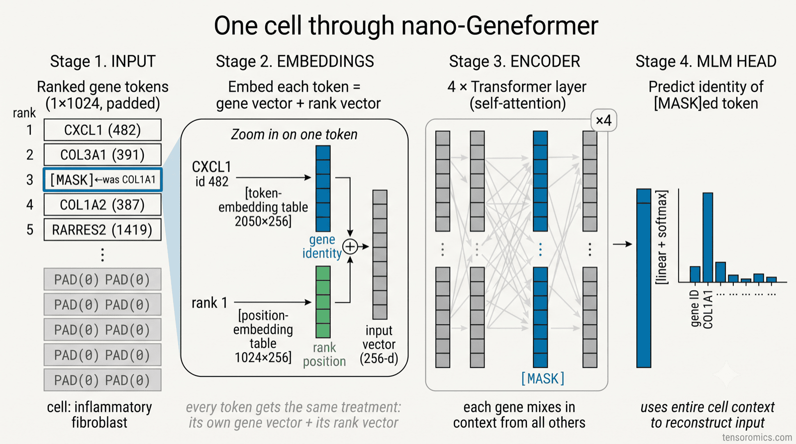
And the code that builds it:
class NanoGeneformer(nn.Module):
    def __init__(self, vocab_size, d_model=256, n_heads=4, n_layers=4,
                 max_len=1024, dropout=0.1, pad_id=0):
        # 1 · token embedding — a gene id becomes a 256-vector (2050 × 256 table)
        self.tok_emb = nn.Embedding(vocab_size, d_model, padding_idx=pad_id)

        # 2 · position embedding — a rank becomes a 256-vector (1024 × 256 table)
        self.pos_emb = nn.Embedding(max_len, d_model)

        # 3 · the encoder — one Transformer layer (self-attention + feed-forward), stacked ×4
        layer = nn.TransformerEncoderLayer(
            d_model, n_heads, dim_feedforward=4 * d_model,
            activation="gelu", batch_first=True, norm_first=True)
        self.encoder = nn.TransformerEncoder(layer, num_layers=n_layers)
        self.norm = nn.LayerNorm(d_model)

        # 4 · MLM head — a 256-vector becomes a score for every gene (256 → 2050)
self.mlm_head = nn.Linear(d_model, vocab_size)Four pieces turn a gene id into a prediction. Let's follow one gene (CXCL1, token id 494, sitting at rank 1 in our fibroblast) through all four. (A fibroblast is a connective-tissue cell that produces the structural collagen proteins of a tissue's scaffolding; this one is inflamed, so inflammatory genes like CXCL1 sit at the very top of its ranked list.)
1 · Token embedding: an id becomes a vector. tok_emb is a lookup table with one learned 256-number row per token id (a 2050 × 256 table, the 2,048 vocabulary genes plus PAD and MASK). Token 494 grabs row 494: a 256-dim vector that is the model's current notion of "CXCL1." Every cell expressing CXCL1 starts from this same vector. Nobody sets those 256 numbers by hand. Across millions of masked-gene guesses, training reshapes the rows (all but the frozen PAD row) so that genes with similar roles drift close together, an effect that sharpens with model size and training, and that a nano model like ours only hints at. It's a word embedding, but for genes.
token 494 (CXCL1) ──lookup──▶ [0.12, −0.41, 0.90, … ] ← 256 numbers(padding_idx=0 pins PAD's row to all-zeros and freezes it, so empty slots add nothing.)
2 · Position embedding: add the rank. A second table, pos_emb, holds one vector per rank slot (1st, 2nd, …). CXCL1 sits at rank 1, so we take that table's rank-1 vector and add it to the CXCL1 vector. The sum encodes both which gene it is and how high it ranks: the only order signal a cell has.
CXCL1 vector + rank-1 vector = the vector that enters the transformerIn symbols, the vector entering the transformer at position is : the gene's own embedding plus the embedding of its rank. Each is a list of 256 numbers (the values shown in the box above). A handy one-number summary of such a vector is its magnitude : how long the arrow is, not how many numbers it holds. For CXCL1 at rank 1, and each have magnitude about 17, and because they point in nearly independent directions their sum has magnitude .
3 · The encoder: genes look at each other. These vectors, one per gene, pass through 4 identical Transformer layers. Each layer does two things: self-attention, where every gene pulls in context from the other genes in the cell (covered in its own section below), then a small feed-forward network: a per-gene transform (widen the 256-vector, apply a nonlinearity, project back down) that lets the model reshape each gene's vector on its own. Both are wrapped in residual connections (each step adds its output onto its input instead of replacing it) and LayerNorm (which rescales each vector to a stable range): standard plumbing that lets you stack layers without training falling apart. Stacking 4 of them means genes attend to genes that have already absorbed context, so structure builds up with depth. (Four is a deliberately small choice: deeper is richer but needs more data and compute. For reference, real Geneformer uses 6 layers, BERT-base 12. It's one line in config.py.) After 4 layers, CXCL1's vector no longer means just "CXCL1"; it means "CXCL1 in a cell full of collagens and inflammatory genes." The rest of the model relies on that contextualized vector.
4 · The MLM head: a vector becomes gene scores. A single linear layer maps each gene's 256-dim vector to 2,050 scores (called logits): one per possible gene. Each score is a dot product of the head's row for gene with the contextualized vector (a dot product multiplies the two 256-number lists entry by entry and sums to a single number, larger when the two align), and softmax turns the 2,050 scores into a probability. At a masked slot, the top-scoring gene is the model's guess.
contextualized vector (256) ──Linear──▶ 2,050 scores ──softmax──▶ P(gene)The shapes, end to end. Watching the tensor change shape as it flows through often makes a transformer click:
input         (64, 1024)         64 cells × 1024 token ids   (integers)
embeddings    (64, 1024, 256)    every id becomes a 256-vector
encoder ×4    (64, 1024, 256)    same shape — vectors, now context-mixed
MLM head (64, 1024, 2050) a score for every gene, at every positionOnly two steps change the shape: the embedding expands each integer into a 256-vector, and the MLM head projects each 256-vector into 2,050 gene scores. The encoder in between leaves the shape untouched: it only rewrites the vectors with context.
The config is deliberately small (d_model=256, n_layers=4, n_heads=4), which comes out to about 4.5M parameters: most of them in the four Transformer encoder layers, with the two embedding tables and the output head making up the rest. Real single-cell foundation models are far larger: tens to hundreds of millions of parameters, trained on tens of millions of cells. This one fits on a laptop.
The forward pass is three lines:
def encode(self, tokens):
    # True where PAD
    pad_mask = tokens.eq(self.pad_id)
    # gene + rank
    x = self.tok_emb(tokens) + self.pos_emb(self.pos_ids)
    # genes look at each other
    h = self.encoder(x, src_key_padding_mask=pad_mask)
    return self.norm(h)

def forward(self, tokens):
    # (B, 1024, 2050) scores
return self.mlm_head(self.encode(tokens))pad_mask tells attention to ignore the PAD slots entirely, so the ~950 empty positions in a typical sparse cell never pollute the real genes.
What goes into the model?
The input is exactly what part 1 produced: for each cell, a ranked list of gene ids, its genes sorted loudest-relative-first (the gene most unusually high for that cell, high relative to that gene's typical level across all cells, at the front), padded to a fixed length. A training batch stacks 64 of these cells into one integer array of shape 64 × 1024, 64 cells (the batch size) by 1,024 rank slots per cell:
batch  shape (64, 1024)
# ranked gene ids, then PAD (0)
cell 0:  [494, 1183, 501, 404, 1450, …, 0, 0, 0]
cell 1:  [ 47, 903,  12, 588,  221, …, 0, 0, 0]
...Why a ranked list rather than raw expression? Two reasons from part 1 carry over. Ranking makes each cell a sequence of discrete tokens, so the whole language-model toolkit applies unchanged. And the order is itself signal: position 1 is the gene most distinctive for the cell, position 2 the next, and so on, so where a gene sits already encodes how important it is (the model reads that rank explicitly, via the position embedding above). That's the entire input: no expression values, no labels. Everything the model knows it has to learn from which gene ids co-occur and in what rank order.
What is self-attention, really?
After the embeddings, each gene in the cell is a 256-dim vector. Self-attention lets each gene update its own vector by looking at every other gene in the cell and pulling in the ones that are relevant to it. A collagen gene in a fibroblast can "see" the other collagens (a family of structural genes fibroblasts express together) and the inflammatory chemokines around it, and fold that context into its representation.
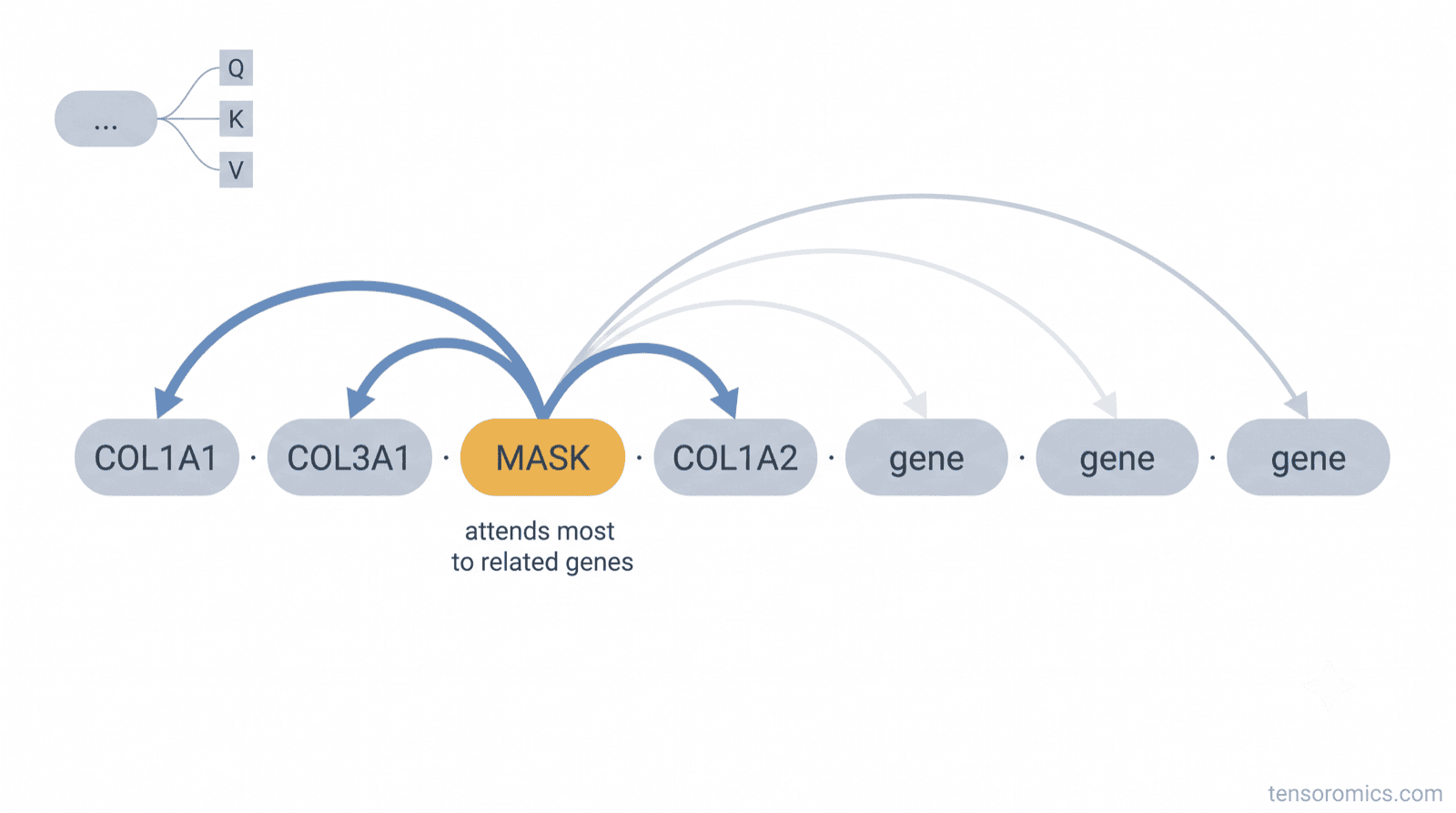
In the picture, the hidden gene leans hardest on the genes it travels with. A trained model's attention is messier than this clean sketch, as the real weights below show.
Mechanically, every gene produces three vectors, each a learned linear projection of its 256-dim vector: a query (what am I looking for?), a key (what do I offer?), and a value (what it contributes when attended to). One gene attends to another by taking the dot product of its query with the other's key, a relevance score. Softmax turns the scores over all genes into weights that sum to 1, and the gene's new vector is the weighted sum of everyone's values:
The just keeps the dot products from getting too large. Do this with 4 heads in parallel (four independent sets of query/key/value), and the layer can track four different kinds of relationship at once (say, "co-expressed with me" in one head, "same rank neighborhood" in another). Stack 4 layers, and genes attend to genes that have already attended to other genes, building up context.
Per gene, that formula means position 's new vector is : a blend of every gene's value vector , weighted by , the softmax weights that sum to 1 (for CXCL1, spread across the cell's 229 genes). So every depends on every gene in the cell, not just gene . The in-silico perturbation in part 5 relies on that.
What it actually does (in the trained model). Rather than trust a single cell, we measure it across many. For 80 held-out fibroblasts (from patients kept out of training) we blank COL1A1 (the same masking trick we train on, coming up in the next section) and record, for every head at every layer, how much of the blank's attention lands on the ECM (extracellular matrix) / collagen neighborhood.
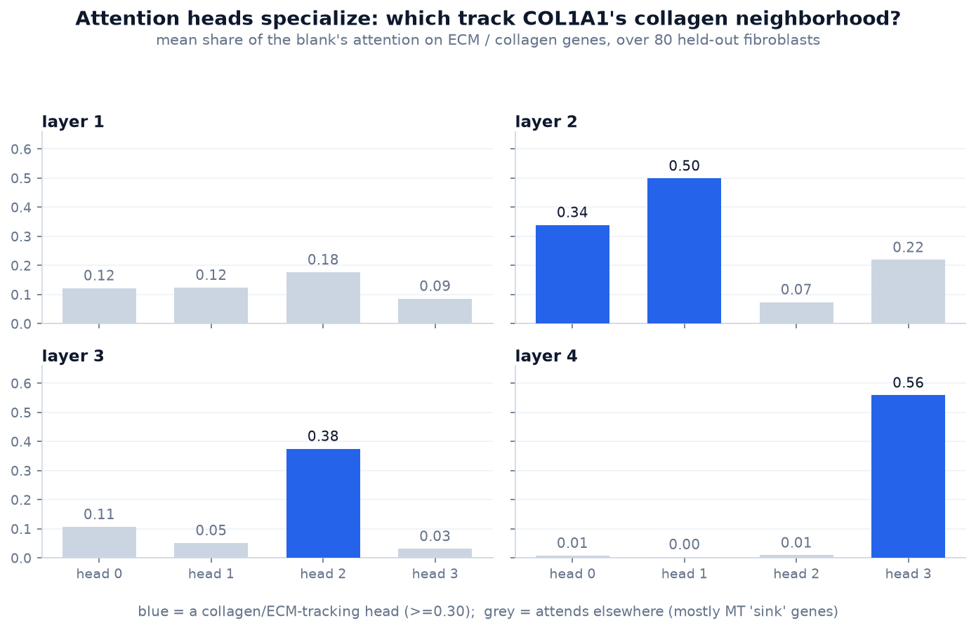
Heads specialize, and the specialization sharpens with depth. Layer 1 is undifferentiated: every head puts about the same modest weight on the collagen neighborhood. Deeper in, specific heads have taken the job: layer 2 head 1 (0.50), layer 3 head 2 (0.38), and most sharply layer 4 head 3 (0.56), which sends over half of a blanked collagen's attention straight to other ECM and collagen genes. That is real co-expression structure, learned from masking alone. But not every head is meaningful: the grey bars are heads that spend their weight elsewhere: mostly on ubiquitous mitochondrial "sink" genes (so common they soak up leftover attention while carrying little specific signal) rather than on the collagen neighborhood. Real trained attention is a mix of the two.
Attention has no built-in left-to-right order and looks at the whole sentence at once, so it naturally learns which genes co-occur, the co-expression structure that defines a cell. (Two flavors of that come up later: a cell's stable type, like fibroblast, in part 3, and its transient state, like inflamed, in part 4.)
Masked-gene prediction: the training task
We met the idea in the primer: hide ~15% of a cell's genes and predict them from the rest, with no labels. That's the entire training signal. Repeated over millions of masked genes, it forces the model to learn the grammar of gene co-expression. Here we make it precise, because one BERT detail matters in practice.
Of the 15% chosen genes, we don't always insert [MASK]. BERT uses 80 / 10 / 10. 80% become [MASK], 10% become a random gene, and 10% are left unchanged:
def mask_tokens(tokens, vocab_size, cfg):
    labels = tokens.clone()
    # 15%
    prob = torch.full(tokens.shape, cfg.mlm_prob)
    # never mask PAD/MASK
    prob[tokens < cfg.N_SPECIAL] = 0.0
    chosen = torch.bernoulli(prob).bool()
    # score only the chosen
    labels[~chosen] = -100

    inp = tokens.clone()
    to_mask = torch.bernoulli(torch.full(tokens.shape, 0.8)).bool() & chosen
    # 80% → [MASK]
    inp[to_mask] = cfg.MASK
    to_rand = torch.bernoulli(torch.full(tokens.shape, 0.5)).bool() & chosen & ~to_mask
    # 10% → random
    inp[to_rand] = torch.randint(cfg.N_SPECIAL, vocab_size, tokens.shape)[to_rand]
    # last 10% left as-is
return inp, labelsIn the code, the first draw (0.8) picks the 80% that become [MASK]; the second (0.5) then splits the remaining 20% evenly: 10% random, 10% left unchanged.
Why the 80/10/10 instead of always [MASK]? Because at test time (parts 3–4) there are no [MASK] tokens: real cells only have real genes. The 10%-random forces the model not to blindly trust every gene it sees, and the 10%-kept forces it to produce the right answer even when the token already looks correct. The labels array holds the true gene only at chosen positions and -100 everywhere else, a sentinel the loss will skip.
What is that loss? For each masked position the model outputs a probability over all 2,050 genes, and the loss is the cross-entropy of the true gene (), averaged over the masked positions. For example, blank CXCL1 in our fibroblast and the trained model gives it probability (about 1 in 280), so that position's loss is . Averaged over all masked genes it lands at ; the next sections read that number against the random-guess baseline and watch it fall.
The training loop
The loop itself is standard, and short (train.py):
for epoch in range(epochs):
    # 64 cells at a time
    for (batch,) in loader:
        # corrupt
        inp, labels = mask_tokens(batch, vocab_size, cfg)
        # (64, 1024, 2050) scores
        logits = model(inp)
        loss = F.cross_entropy(logits.view(-1, vocab_size),
                               labels.view(-1), ignore_index=-100)
        opt.zero_grad(); loss.backward()
        # stability
        nn.utils.clip_grad_norm_(model.parameters(), 1.0)
opt.step(); sched.step()Each step is five moves:
- Corrupt the batch with
mask_tokens. - Forward it through the model → a score for every gene at every position.
- Score with cross-entropy, but only at masked positions, since
ignore_index=-100tells it to skip everything else. - Backprop (
loss.backward()) computes, for every weight, which way to change it to lower the loss (the gradients). - Step the optimizer to apply those changes: the gradient-descent update from the primer, nudging every weight toward a better next guess.
A few standard knobs keep it stable: AdamW adapts each weight's step size; the learning rate warms up over the first ~125 steps and then cosine-decays to zero (ease in gently, settle down at the end); and gradient clipping caps the update size so no single batch can blow up the weights.
Watching it learn
One command runs the whole thing, python train.py --epochs 2 (two full passes over the training cells), and the loss prints each step. Here's that 2-epoch run on the ~80k training-split cells (of a 100k-cell subsample, with whole patients held out; Apple Metal GPU, ~3 hours):
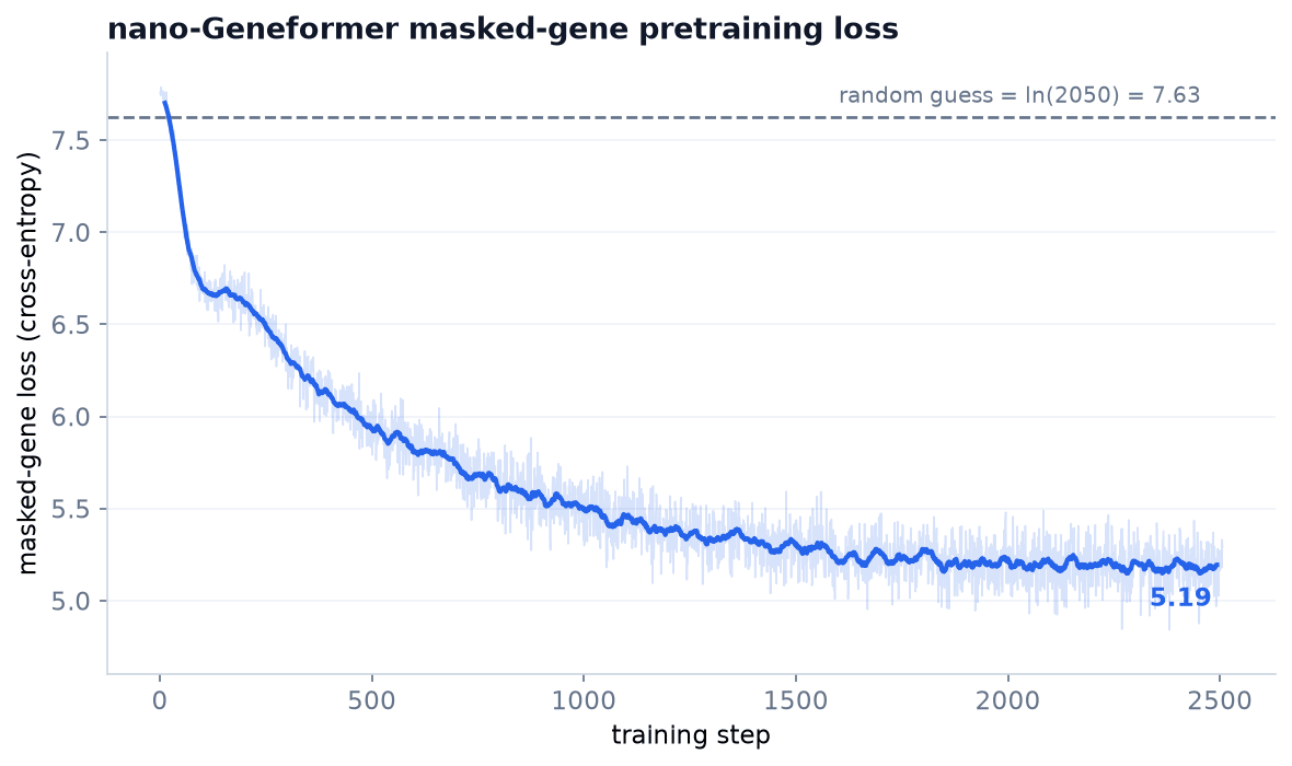
Read it against one anchor. With 2,050 possible genes, a model guessing at random scores a cross-entropy of , the dashed line. The curve starts just above it, at about 7.76 (an untrained head is a hair worse than uniform), confirming the model begins knowing essentially nothing, then:
- drops sharply in the first ~100 steps to ~6.6: it quickly learns the easy statistics (which genes are common, which never co-occur),
- then declines steadily through both epochs to about 5.19. In plain terms, its effective guess narrowed from 1-in-2,050 toward roughly 1-in-180. (Because the loss is , is the effective number of equally likely genes it is choosing among, so .) Narrowing it that far means the model has picked up which genes co-occur, from the masking signal alone.
- The fuzz is normal: every step sees different cells with a different random 15% masked.
For calibration: a curve that stayed flat near 7.6 would mean the model isn't learning at all; one that dipped and then climbed back up would signal training instability, usually a learning rate set too high. (Overfitting wouldn't show up on this plot at all: it drives the training loss steadily lower while performance on held-out cells gets worse, so you can only catch it with a separate validation loss, not this training curve.) Ours drops and holds, the shape of healthy pretraining.
Lower loss isn't the goal in itself. The goal is reading held-out biology off the embedding (parts 3 and 4). But a loss that falls this far means the encoder learned something worth testing. The run saves two files in checkpoints/: model.pt (the trained weights) and loss_history.npy (the per-step loss the curve above was drawn from).
Can nano-Geneformer predict a masked gene?
The loss curve is indirect evidence. The direct test is to do at inference exactly what we did in training, but on a cell the model never saw. Take a held-out cell (a patient kept out of training entirely), blank one gene with [MASK], run the model forward, and read the top-scoring gene off the head. Because BERT is bidirectional, it fills the blank using every other gene in the cell: the ones ranked above and below.
Here is one held-out goblet cell (a mucus-secreting cell of the gut lining) with a mid-ranked gene hidden:
FCGBP > ITLN1 > CLCA1 > [MASK] > …        true gene:  TFF3
model's #1 guess: TFF3 (11%) FCGBP, ITLN1, CLCA1, TFF3 = goblet mucus genesShown three goblet-cell mucus genes, the model fills the blank with another one, TFF3. It isn't reciting a memorized cell; it's placing probability on the right biological neighborhood. The effect is sharpest for genes locked into a tight co-expression module. Hide the top gene of a held-out plasma cell and it recovers the immunoglobulin IGHA1 at 93%: every runner-up (IGLC3, IGLC2, IGHA2) is also an immunoglobulin. A dendritic cell's CD74 (the MHC class II invariant chain, part of the machinery immune cells use to display antigens) comes back at 87%, rebuilt from its co-expressed MHC-II partners. A fibroblast's CXCL14 (a different chemokine from the CXCL1 we followed earlier) returns at 50%, with the stromal genes ADAMDEC1 and CFD close behind.
Where it's reliable: the easy wins. Masking genes across 400 held-out cells and ranking by how often the model recovers the exact gene, the top of the list is unsurprising:
| gene | top-1 recovery | what it is |
|---|---|---|
MT-CYB, MT-ND4, MT-RNR2 | 72–76% | mitochondrial: present in nearly every cell |
FTL, FTH1 | 65–67% | ferritin: near-ubiquitous |
FABP1, KRT8, LGALS4 | 32–55% | epithelial identity genes |
IGHA1 | 38% | immunoglobulin: defines plasma cells |
They are easy for two different reasons, and both come down to low uncertainty about what fills the blank:
- Sheer frequency. Mitochondrial and ferritin genes are expressed in almost every cell, so before reading any context the model already knows a blank is often one of them, the way a text model fills a blanked "the" or "of" easily. And because they are everywhere, when you hide one, its equally ubiquitous partners are still visible in the same cell, pointing right at it.
- Tight co-expression. A plasma cell is an antibody factory: most of its transcriptome is immunoglobulin. Blank one immunoglobulin and the rest of the cell still shouts "plasma cell" from every other slot, so the missing gene is nearly determined by everything around it.
The middle-of-the-ranking genes have neither advantage: not common enough to guess blind, not locked into a tight module that pins them down. The model spreads its probability thin and usually misses. Most of the errors come from those middling genes.
Why the MT- genes rank so high, and only half of it is technical. They are ubiquitous (the frequency effect above), but in this colon atlas they are also partly cell-type signal: colonic epithelium (the sheet of lining cells of the gut) is metabolically dense (those cells run energy-hungry absorption and transport) and mitochondria-rich. Part 1 works through the tissue-aware QC this rests on (Geneformer's adaptive per-sample filter, which removes dying cells but deliberately keeps that healthy high-mito epithelium), so here the MT- tokens carry real biology, not just noise.
Across those same held-out positions:
- top-1 accuracy: 7.1%, the exact gene, out of 2,048, on the first guess,
- top-5 accuracy: 16.1%, the true gene somewhere in the top five.
Against a 1-in-2,048 chance rate (0.05%), 7% is roughly 140× better than random: real, learned structure, not luck. But 7% is also modest. This is a 4.5M-parameter model trained on ~80k cells (the QC'd training split of a 100k-cell subsample) for two epochs on a laptop GPU, not the 30-million-cell Geneformer. It learned the high-frequency co-expression grammar (the common genes, the tight lineage families) cleanly, and the rest only faintly. (The script is predict_masked.py in the repo.)
What you get at the end
Training leaves the trained weights in checkpoints/model.pt (with a loss_history.npy log beside it), but that one model exposes several different views of a cell. You pretrain to get them. Each is useful either for diagnosing whether the model learned anything, or for reusing it on a new task.
| Output | Shape | What it is | Good for |
|---|---|---|---|
| Gene embeddings | 2050 × 256 | one fixed vector per gene (tok_emb), context-free | gene–gene similarity |
| Contextual gene vectors | cells × 1024 × 256 | one vector per gene per cell, after attention (encode) | per-gene, context-aware tasks |
| Cell embeddings | cells × 256 | those vectors mean-pooled over each cell's genes (cell_embedding) | clustering, classification, disease prediction |
| Attention maps | 4 × 1024 × 1024 | which genes attend to which, per head (× 4 layers) | interpretability |
| Masked-gene predictions | cells × 1024 × 2050 | a gene distribution at every slot (forward) | imputation, in-silico perturbation |
Two of these we have already seen: we plotted the attention maps to watch heads specialize, and the masked-gene predictions filled in TFF3 and IGHA1. The same trained model hands you both per-gene and per-cell representations, for free. Two of them carry the rest of the series:
- Cell embeddings are the workhorse: one 256-vector per cell, computed without any label. It is the mean of the cell's contextualized gene vectors, , over the cell's real genes; for our fibroblast, vectors average into a single 256-vector of length about 9. You can cluster, classify, project to 2-D, or search these. Part 3 puts them to the test: can they name a cell's type on a held-out patient? Part 4 asks the harder question: disease.
- Gene embeddings are the natural diagnostic. If pretraining worked, collagens should sit near collagens in that
2050 × 256table. For our small model they mostly don't yet (COL1A1's nearest neighbours are a grab-bag, not other collagens), which is one of the things part 4 tries to fix, by tying the gene embeddings to the prediction head: reusing one table for both, so the two are forced to match.
And the masked-gene head has a second life beyond training: delete a gene from a cell, run the model, and watch how the predicted distribution shifts, an in-silico perturbation (perturb.py in the repo) that asks which genes, if silenced, nudge a cell toward a healthier profile.
What we built
We began with a cell as a bag of ~20,000 gene counts and ended with a 4.5M-parameter BERT that reads it as a ranked sentence. The model trained on a single task (fill in genes hidden at random) and was never shown a cell-type or a disease label. To do that task at all, it had to learn which genes travel together, and the fill-in-a-blank test confirmed it did: on held-out patients it recovers common and lineage-defining genes reliably, and even its misses land in the right biological neighborhood.
Self-supervised pretraining buys you the several reusable representations above (gene, cell, attention, prediction), each obtained without ever defining a fibroblast or an inflamed biopsy.
Whether that representation is useful is a separate question, and not a given. A falling pretraining loss proves the model learned something; it does not prove it learned the thing you care about. Part 3 runs the first test: freeze the model, average each cell's gene vectors into one embedding, and ask a simple linear classifier to name the cell's type, then race it against plain PCA. Part 4 pushes to the harder target, disease state, where the result is mixed. The reason goes back to a decision from part 1: what rank encoding chose to throw away.