Geneformer from scratch, part 1: a cell is a sentence

Single-cell RNA sequencing (scRNA-seq) measures how strongly each gene is expressed in one cell at a time — not just which genes are on, but how much — across tens of thousands of cells at once. In 2023, Geneformer showed that this data could be treated the way modern AI treats language: pretrain one transformer on millions of cells, with no labels, and it absorbs a general-purpose "grammar" of gene regulation that transfers from one task to the next. It was one of the first foundation models for single-cell biology.

This series builds a tiny, from-scratch version of Geneformer — small enough to pretrain on a laptop in an afternoon, but with every real piece in place: the tokenizer, a BERT-style transformer, masked-gene pretraining, and the probes that ask what it learned. We run the whole thing on a real ulcerative-colitis (UC) atlas of 365,492 cells (Smillie et al. 2019), and by the end we probe it for inflammatory-bowel-disease (IBD) biology.

Four parts:

1. A cell is a sentence — this post — getting started: turn raw expression into rank-ordered gene tokens.
2. Build and train the BERT — the transformer, and masked-gene pretraining.
3. Test it — does the learned representation know disease? Probe it against a classical baseline.
4. Scale it up — more data, or better tokens?

All the code lives in one place — nano-geneformer-ibd on GitHub. Clone it and follow along.

This first part is about the representation. Before there is any model to train, you have to turn a cell into something a transformer can read. Geneformer's answer: turn a cell into a sentence.

A large language model reads a sentence — an ordered list of words — and learns which words keep each other's company. Geneformer plays the same game on cells:

• a cell is a sentence,
• a gene is a word,
• and the word order is the ranking of a cell's genes by how strongly it expresses them, relative to how strongly cells normally express them.

So each cell becomes a ranked list of gene tokens — GENE_A > GENE_B > GENE_C > …, loudest first. That ranked list is the entire input to the model.

Why a ranked list of gene tokens?

A cell's expression is fundamentally quantitative — thousands of genes, each with a number. Compressing all of that to "gene A ranks above gene B" throws real information away. So why do it?

Because it makes a cell look exactly like a sentence. Once a cell is a sequence of discrete tokens, it is structurally identical to a sentence of words, and you can lift the entire language-model toolkit unchanged: token embeddings, positional encoding, self-attention, and — crucially — masked-token pretraining, the same objective that trained BERT. No custom architecture, no bespoke loss. For Geneformer, that reuse was the point: the mature NLP toolkit could be applied to cells with almost no changes.

The cost is magnitude. Ranking keeps which genes are high and drops how high. Two cells can share the same gene ordering yet differ ten-fold in how strongly they express those top genes, and a rank encoding can't tell them apart. Feeding the raw quantitative values would keep that signal, but it is genuinely harder: continuous numbers don't slot into a fixed token vocabulary, so you need extra machinery — value-binning or learned value embeddings — plus more care to keep training stable.

But the ordering still carries most of the biology. A cell's identity lives mostly in which genes are on and which dominate. A cell type is a gene program: a cytotoxic T cell runs the T-cell program (CD3E, TRBC2, GZMA…), a plasma cell the antibody program (immunoglobulins), a fibroblast the collagen program. Two cells of the same type run the same program, so they push the same genes to the top of their sentences in roughly the same order — same-type cells look alike to the model and different types look different, which is exactly the structure it needs to learn. What's lost with magnitude is finer detail (how strongly a program runs — say, how inflamed a cell is), not the cell's basic identity.

Advanced models add the magnitude back. Much of the progress in single-cell foundation models since Geneformer is really about how to feed expression values, not just gene identity:

• scGPT pairs each gene token with a binned expression-value token — the model sees both which gene and roughly how much.
• scBERT gives each gene a gene embedding plus a discretized expression embedding (expression bucketed into levels).
• scFoundation goes further and reads continuous expression values directly, with a read-depth-aware objective.

We start where the field started — pure rank — because it's the clearest way to see the whole machine end to end. In part 4 we'll measure exactly what that simplicity costs on a real disease task, and whether adding magnitude back is worth the complexity.

The rest of this post builds that ranked list — the rank encoding — in three moves.

• Normalize. Put every cell on the same scale first. A cell that was simply sequenced more deeply (more transcripts captured) shouldn't look more active than its neighbor; we want the differences that survive to be biological, not technical. The standard fix is to rescale every cell to the same total count.
• Pick a vocabulary. Keep only the ~2,000 genes worth modeling — the ones that actually vary from cell to cell — so every cell is described in the same fixed set of "words." The genes that are high in every cell (housekeeping) carry no identity, so they're dropped here.
• Rank. For each cell, compare each of its genes to how high that gene usually runs across all cells, then sort from most to least unusually-high. "Against its own baseline" just means measured relative to its own typical level — so a gene comes first if it's surprisingly loud for this cell, not merely loud in general. That ordered list is the sentence the model reads.

The next sections do each move on the real UC data.

The rank-encoding recipe

The data-prep script (prepare.py) does six things:

1. Load the atlas into one cells-by-genes matrix.
2. QC filter — drop weak cells and barely-seen genes.
3. Normalize every cell to the same total — 10,000 counts (CP10k) — so a deeply- and a shallowly-sequenced cell compare fairly.
4. Pick a vocabulary — the 2,048 most variable genes. (Housekeeping genes barely vary, so they don't make the cut — they're excluded from the vocabulary entirely.)
5. Median-scale, then rank each cell's genes. ← the idea
6. Split by patient and save.

Steps 1–3 are standard preprocessing, which we'll skip here. Let's walk steps 4 through 6 — the moves that decide what the model actually sees.

Pick a vocabulary

A transformer needs a fixed vocabulary — the same set of "words" available to every cell. But we can't make every gene a word: the human genome has roughly 20,000 protein-coding genes (this atlas measures about 18,000 of them), and carrying them all would bloat the model while adding mostly noise, since most genes are undetected or uninformative in any one tissue. So we keep only the informative subset — the 2,048 most variable genes, the ones whose expression changes the most from cell to cell. A gene that barely varies (housekeeping again) can't help tell cells apart, so it never enters the vocabulary. Sparsity makes a small vocabulary especially natural here: scRNA-seq matrices are mostly zeros — any single cell has no counts at all for the large majority of genes (part true biological silence, part technical dropout) — so keeping just the ~2,000 informative genes discards very little real signal.

sc.pp.log1p(adata_log)                                    # log-scale for this step
sc.pp.highly_variable_genes(adata_log, n_top_genes=2048)  # the 2,048 vocabulary genes
adata = adata[:, adata_log.var["highly_variable"]]        # keep only those genes

The same step also computes a 50-dimensional PCA of these genes — a standard linear summary of each cell. That isn't part of the model; it's the baseline we'll race the model against in part 3, to see whether pretraining learned anything a simple linear method didn't.

sc.pp.pca(adata_log, n_comps=50, use_highly_variable=True)  # the PCA baseline

The median trick: rank a gene against its own baseline

Picking the vocabulary already dropped the steady housekeeping genes — so isn't ranking solved? Not quite. Choosing variable genes doesn't put them on equal footing: among the 2,048 survivors, typical expression still ranges from about 0.5 to 64 — over 100×. So ranking by raw expression would let the naturally high-abundance genes sit on top of every cell, telling you little about any one of them. We want each cell's distinctive genes at the top instead — the ones that are unusually high for that cell. The fix is to score each gene against its own typical level.

(Picking the vocabulary is like dropping stopwords; dividing by the median is the IDF half of TF-IDF — down-weight the globally loud so a normally-quiet gene being loud counts for more. You need both.)

First, compute each gene's "normal" level — the median of its nonzero values across cells:

for j in range(n_genes):                       # each gene
    col = X.data[X.indptr[j]:X.indptr[j+1]]    # the cells that express it
    gene_median[j] = np.median(col)            # its typical level

Then, for each cell, we divide its counts by that per-gene baseline and rank:

vals  = counts / gene_median[expressed_genes]  # loudness relative to normal
order = np.argsort(-vals)[:1024]               # sort high -> low, keep top 1024
tokens = expressed_genes[order] + 2            # gene index -> token id (0=PAD, 1=MASK)

The one line to read slowly is vals = counts / gene_median. A gene ranks high in a cell only if its score

$\text{score} = \frac{\text{count}}{\text{median}}$

is large — where count is the gene's expression in this cell and median is its usual level across cells. It's loud for itself, not just loud in absolute terms. That single division demotes the high-baseline genes (loud in general, so unremarkable once divided by their own high baseline) and promotes the genes that are distinctively high in this cell.

A worked example. Say four genes have typical levels [2, 5, 10, 1], and a cell expresses three of them with counts [6, 20, 1]:

gene            g0     g2     g3
count            6     20      1
typical level    2     10      1
score = /median  3.0    2.0    1.0     ->  ranked  g0 > g2 > g3

Notice g2 had the biggest raw count (20) but loses to g0. Its baseline is high (10), so a count of 20 is unremarkable for it; g0's count of 6 against a baseline of 2 is the real signal. By raw counts the order would be g2 > g0; the median flips it. That flip is the whole point.

Does the ranking recover real biology?

Rank 1 is the first token in a cell's sentence — the single gene that scored highest against its own baseline in that cell. If the median trick is doing its job, the genes that most often land in that top slot should be recognizable cell-type markers, not housekeeping genes. So let's count, across 100,000 UC cells, which gene wins rank 1 most often:

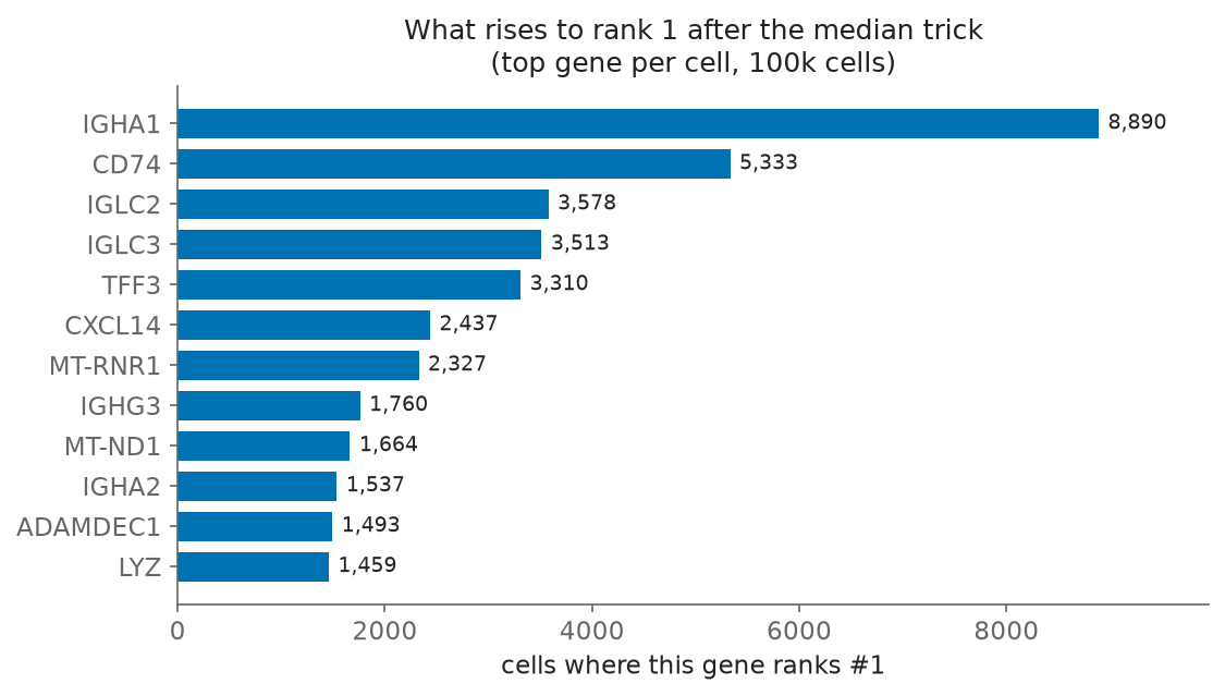
Most are recognizable cell-type markers: the immunoglobulins (IGHA1, IGLC2, IGHG3) mark antibody-secreting plasma cells; CD74 marks antigen-presenting cells; TFF3 marks goblet cells; LYZ marks myeloid cells. The two mitochondrial genes (MT-RNR1, MT-ND1) are the honest exception — they flag metabolically active or stressed cells rather than a cell type, a reminder that ranking surfaces whatever dominates a cell, biology and quality alike. But the dominant signal is clearly cell identity, from ranking alone.

And a single cell makes it vivid. Here is one real cell, rank-encoded, straight from the pipeline:

cell type: Inflammatory Fibroblast   (label: Inflamed)
sentence:  CXCL1 > COL3A1 > COL1A1 > COL1A2 > RARRES2 > … > MMP2 > …

Nobody labeled this cell. Ranking its genes surfaced the identity on its own: the collagens (COL1A1, COL1A2, COL3A1) that make it a fibroblast, and at the very top CXCL1, an inflammatory chemokine, with MMP2 (tissue remodeling) a few positions down. That matches the biology of inflamed IBD stroma.

Why split by patient, not by cell?

Before saving, we assign each cell to train or validation — by patient, never by cell:

uniq = sorted(set(patients))            # the unique patients
val_patients = set(uniq[::5])           # hold out every 5th patient
split = ["val" if p in val_patients else "train" for p in patients]

Cells from one patient share that person's genetics and batch quirks. Split cells at random, and a model can "predict disease" by secretly recognizing which patient a cell came from — memorizing the batch instead of learning biology. Holding out whole patients prevents this, so the probe in part 3 measures real generalization, not memorized batch.

The tokenized dataset

Running prepare.py on a 100,000-cell subsample of the atlas (the full 365k works too, just slower) writes five files to data/:

tokens.npy   (100000, 1024)  int64   every cell as a ranked gene sentence (PAD = 0)
pca.npy      (100000, 50)     float   the classical baseline for part 3
vocab.json   2,050 tokens             2,048 genes + PAD + MASK
gene_median.npy, meta.npz             per-gene baselines; labels / patient / split

patients: 30 total, 6 held out  ->  80,313 train / 19,687 val cells
labels:   Healthy / Inflamed / Non-inflamed

And here is what a single row actually looks like — cell 1, the inflammatory fibroblast from earlier, straight off disk:

tokens[1] = [482, 391, 386, 387, 1419, 1469, 1154, …, 843, 890, 0, 0, 0, …]
            └──────────── 201 ranked gene tokens ───────────┘└─ PAD to 1024 ─┘

decoded   =  CXCL1 > COL3A1 > COL1A1 > COL1A2 > RARRES2 > RNA18S5 > MMP2 > …

Each integer is a gene's token id — vocab.json maps 482 → CXCL1, 391 → COL3A1, and so on — sorted loudest-relative-first, then right-padded with 0 (PAD) out to 1,024. Note only 201 of the 1,024 slots are used: cells are sparse. The whole dataset is 100,000 integer rows like this.

Why pad at all? A transformer processes a batch of cells at once as a single rectangular array, so every row has to be the same length. Cells express different numbers of genes, though — this one has 201, another might have 400 — so we fix the length at 1,024: shorter cells have their empty slots filled with a placeholder token, PAD (id 0), and the rare cell with more than 1,024 detected genes keeps just its top 1,024. In part 2 the model is told which positions are PAD and skips them (an attention mask), so padding never changes the answer — it only makes the rows line up into one array.

tokens.npy is the entire input to the model — 100,000 cells, each a ranked list of up to 1,024 gene tokens. In part 2 we build the tiny BERT that reads these sentences and pretrain it by hiding genes and asking it to guess them back (masked-gene prediction), then watch the loss fall on a laptop GPU.