Notes
Spatial transcriptomics of Crohn's disease: cell segmentation errors in Xenium data
Even with several classes of biologic drugs available, many patients with Crohn's disease still need surgery. One reason may be the inflammatory fibroblast. An expansion of these cells is linked to resistance to corticosteroids, anti-TNF, and anti-integrin drugs (Friedrich et al., 2021; Thomas et al., 2024). We still don't know where these cells come from, or whether a fibroblast that becomes one stays that way.
Koplev et al. (Nature Immunology, 2026) set out to answer both questions, and I liked how they did it. They started from an observation in their spatial transcriptomics data and ended with a drug test. At each step they added a new kind of data:
spatial transcriptomics → single-cell RNA + ATAC → fibroblasts in a dish → an existing cancer drug → gut-on-a-chip
We start with the first step, their spatial transcriptomics data, and explore it in Python.
Spatial transcriptomics of Crohn's disease, a series:
- A first look: load the atlas in Python and zoom from whole sections into an ulcer.
- Cell segmentation errors in Xenium data (this note): how close the cells are packed, and whether genes from one cell type show up in the cells next to it.
The atlas holds 2.1 million cells from 16 pieces of Crohn's disease ileum, from eight patients. In the ulcer we zoomed into in part 1, the inflammatory fibroblasts are found among immune cells.
Xenium detects each RNA molecule as a dot and reads which gene it comes from. But we don't know which cell the dot came from. To count genes per cell, we first have to find each cell and trace its outline. This step is called segmentation. It is hard to get right, because the edge between two cells is often not clear in the stain images. For this atlas, the authors used Xenium's own segmentation, a deep-learning model from 10x Genomics. As we saw in part 1, it tries three ways to find each outline, in this order:
- From a boundary stain that marks cell membranes: 17% of the cells in this atlas.
- From an interior stain, when the boundary stain is not clear enough: 80%.
- By growing the nucleus outward by 5 µm, when neither stain is clear enough: 3%.
Then, for each cell, Xenium counts the dots of each gene that fall inside its outline. These are the cell's gene counts. All three ways work from the stain images alone. They don't use where the RNA molecules (the dots) were detected, so an outline can't be adjusted to fit the RNA of its own cell.
Counting this way works well when cells are far apart. In the gut, many cells touch. The 150 µm patch in part 1, for example, held 459 cells. Near the edge between two cells, a dot from one cell can land inside the other cell's outline, and it is then counted for the wrong cell.
Figure 1. How dots become gene counts, and how a dot gets counted for the wrong cell
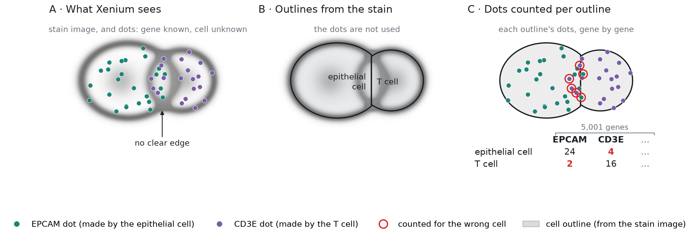
To keep the figure simple, each cell shows the dots of one gene only. In the atlas, every cell is counted this way for all 5,001 genes on the panel. The table under panel C is a small piece of the result, the count matrix.
How often does that happen, and does it change the counts? To check directly, we would need what panels A and B of Figure 1 show: the position and gene of every dot, and the outline of every cell. Then we could look for dots like the ringed ones in panel C, such as an EPCAM dot inside a T cell's outline, right at the edge with an epithelial cell.
The authors didn't share the dots or the outlines, so we can't see which dots were counted for the wrong cell. They shared two tables, with one row for each of the 2.1 million cells, in the same order. Figure 2 shows a few real rows of each:
- The cell table gives each cell's center (x and y, in µm), its area, and its cell type.
- The count matrix is the result of panel C in Figure 1. It has one column per gene, and each entry is the number of dots of that gene in that cell.
Figure 2. The data we work with: the cell table and the count matrix, one row per cell
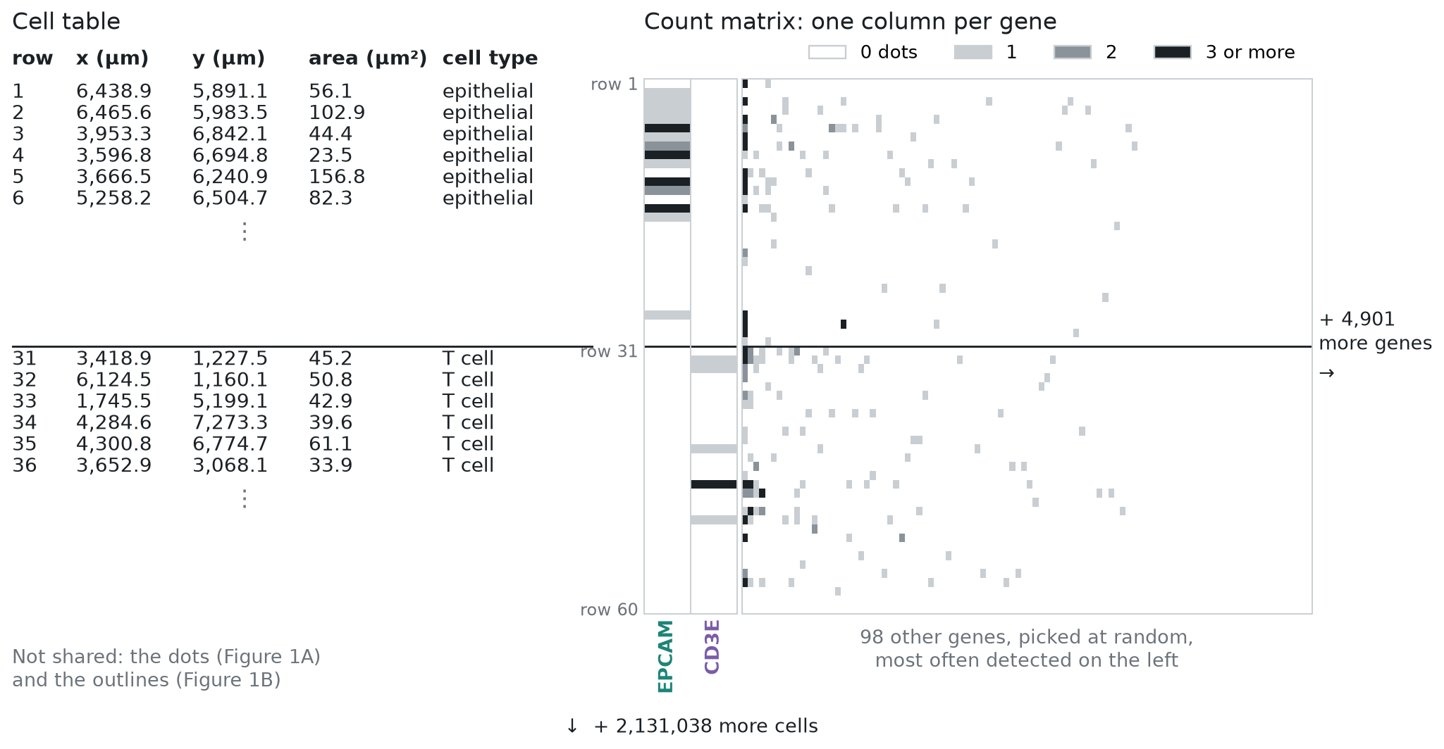
The 60 cells in Figure 2 come from one inflamed section: 30 epithelial cells and 30 T cells. The matrix shows 100 of the 5,001 genes. White means no dots, and most squares are white. A typical cell in this atlas holds 149 dots, spread over 131 genes, so most genes are 0 in most cells. Across the whole matrix, 96.8% of the entries are 0. Even EPCAM is 0 in many of the epithelial cells here. With counts this small, a single dot counted for the wrong cell matters. One EPCAM dot in a T cell is as much EPCAM as a typical epithelial cell holds.
In this note, we use only what they did share to ask how often cells are close enough for this to happen, whether it shows in the counts, and what it does to an analysis. We do it in four sections, each a few blocks of Python:
- How close are the neighboring cells? From each cell's center and area, we measure how far away its nearest cell is, and whether the two are close enough to touch.
- Are neighbors the same cell type? From the cell types, we check how often touching cells are different types. An RNA molecule counted for the wrong cell matters most then.
- Do cells hold genes from the cells next to them? EPCAM is made by epithelial cells, so a T cell or a fibroblast should hold almost no EPCAM RNA. If RNA molecules are counted for the wrong cell, the non-epithelial cells right next to epithelial cells will hold some EPCAM, and those far from any epithelial cell won't. From the gene counts, we compare the two. Then we repeat the test with a marker gene for each of the other cell types.
- Does it change what we learn about T cells? We compare T cells next to the epithelium with T cells deeper in the tissue, the way a differential expression analysis would, and look at which genes come out on top. All of the top 20 are epithelial genes.
How close are the neighboring cells?
Let's start coding. First we load the cell table, as in part 1. The data file is an .h5ad file,
which we open with h5py and read one column at a time. That way we load only what we need, and the
9 GB count matrix stays on disk until section 3. We keep nine columns and give them short names:
where each cell is (section, x, y), how big it is (area), how many RNA molecules (dots) it holds in
the count matrix (dots), its cell type at two levels of detail (cell_type, fine_type), how sure the authors' classifier
was of that type (confidence), and its dots from negative-control probes, which match no gene (controls). We use the
last two in the checks of section 3:
Show code: load the cell table (from part 1)
import h5py
import numpy as np
import pandas as pd
import matplotlib.pyplot as plt

# open the file; we read only the cell table (obs), the 9 GB matrix stays on disk
f = h5py.File("xenium5k_scVI_CellCharter_batch2_reannot_SCP.h5ad", "r")
obs = f["obs"]

def column(name):
    g = obs[name]
    # numbers are stored as plain arrays: read them as is
    if isinstance(g, h5py.Dataset):
        return g[:]
    # labels are stored as codes plus a list of categories: turn codes into names
    return g["categories"].asstr()[:][g["codes"][:]]

# short names (left) for the columns we need (right), one row of `cells` per cell;
# dots is n_counts, the cell's RNA molecules summed over all genes in the count matrix
# (transcript_counts is a little higher, because it also counts molecules not in the shared matrix)
cols = {"section": "biosample_id", "x": "x_centroid", "y": "y_centroid",
        "area": "cell_area", "dots": "n_counts",
        "cell_type": "megagut_lvl1_majority_voting", "fine_type": "megagut_lvl3_majority_voting",
        "confidence": "megagut_lvl1_conf_score", "controls": "control_probe_counts"}
cells = pd.DataFrame({short: column(name) for short, name in cols.items()})

# number of cells (rows) and columns
print(cells.shape)(2131098, 9)We measure how close the cells are in three steps, shown in Figure 3:
- For each cell, find the cell whose center is closest, and the distance d between the two centers.
- Draw each cell as a circle with the same area. The shared data has each cell's area but not its outline, so we assume that each cell is round. A circle with the same area has radius r = √(area / π).
- The two circles overlap when d is less than the sum of their radii.
In Figure 3, d is 6.7 µm, and the two radii add up to 4.4 + 3.6 = 8.0 µm, so cell A overlaps its nearest cell, B.
Figure 3. How we decide that a cell overlaps its nearest cell
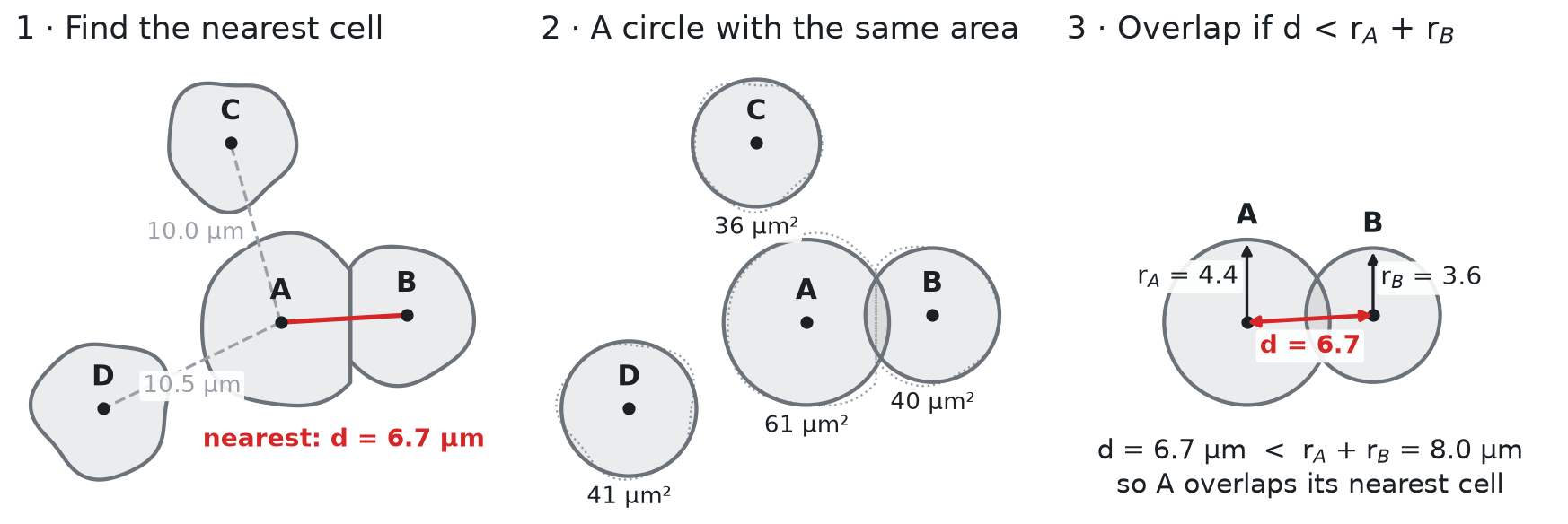
The round shape is an assumption, and it has drawbacks. Real cells are not round. Fibroblasts are long and thin, and epithelial cells are tall columns. For a long cell, the circle reaches too far across the cell and not far enough along it. So the test can call two cells touching when a small gap separates them, and it can miss two long cells that touch end to end. The errors go both ways, so the share of touching cells we get is an estimate. Also, we test each cell only against its nearest cell, while a real cell can touch several. With the real outlines, we could instead check which outlines share an edge. This atlas doesn't have them, but in Figure 5 we run that check on a public sample made the same way.
Step 1 is a nearest-neighbor search on the cell centers (x, y, in µm). Comparing every cell
with every other cell in the same section would mean billions of distances. A k-d tree avoids
that. It splits the section into smaller and smaller boxes, once, so that for each cell it only
needs to check the cells in the nearby boxes. In spatial omics, the usual tool is
squidpy.gr.spatial_neighbors from Squidpy, which links each cell
to its 6 nearest cells by default. We need only the single nearest cell, so we use SciPy's k-d tree,
cKDTree, directly.
We run the search one section at a time, because each section has its own coordinates. For each
cell, we keep two things: the distance to its nearest cell (nn_dist), and the row number of that
cell (nn), so that we can look up the neighbor's size and type later:
Show code: find each cell's nearest neighbor
from scipy.spatial import cKDTree

# the cell centers, as an array with one row per cell and two columns (x, y)
xy = cells[["x", "y"]].to_numpy()

# for each cell: distance to its nearest cell, and that cell's row number
nn_dist = np.zeros(len(cells))
nn = np.zeros(len(cells), dtype=int)

# `rows` holds the row numbers of the cells in one section
for section, rows in cells.groupby("section").indices.items():
    # build the tree from this section's centers, then ask for the 2 closest centers to each cell;
    # the closest is the cell itself (distance 0), the second is its nearest neighbor
    dist, j = cKDTree(xy[rows]).query(xy[rows], k=2)
    nn_dist[rows] = dist[:, 1]
    # j counts within the section; rows[j] turns it back into a row number of `cells`
    nn[rows] = rows[j[:, 1]]
cells["nn_dist"] = nn_dist
cells["nn"] = nnSteps 2 and 3 need each cell's radius, which we compute from its area. Then we compare the distance to the nearest cell with the two radii, and print the typical distance and size:
Show code: compare distances with cell size
# radius of a circle with the same area as the cell
r = np.sqrt(cells.area.to_numpy() / np.pi)
cells["diameter"] = 2 * r

# a cell overlaps its nearest neighbor when the two circles overlap;
# r is the cell's own radius, and r[nn] is the radius of its nearest neighbor
cells["overlaps"] = cells.nn_dist < r + r[nn]

# the median is the middle value: half the cells are below it, half above
print(f"median distance to the nearest cell: {cells.nn_dist.median():.1f} µm")
print(f"median cell diameter: {cells.diameter.median():.1f} µm")
print(f"cells that overlap their nearest neighbor: {cells.overlaps.mean():.0%}")

# the same share, section by section (the lowest and the highest of the 16)
by_section = cells.groupby("section").overlaps.mean()
print(f"per section: {by_section.min():.0%} to {by_section.max():.0%}")

# how much the share depends on the circle size: every radius 10% smaller, then 10% larger
for scale in [0.9, 1.1]:
print(f"radii x {scale}: {(cells.nn_dist < scale * (r + r[nn])).mean():.0%} overlap")median distance to the nearest cell: 6.1 µm
median cell diameter: 7.4 µm
cells that overlap their nearest neighbor: 76%
per section: 52% to 90%
radii x 0.9: 62% overlap
radii x 1.1: 84% overlapA typical cell is 7.4 µm across, but its nearest neighbor is only 6.1 µm away, center to center. Three cells in four overlap their nearest neighbor as circles, and in every section at least half do. Xenium's outlines themselves never overlap, because each point of the image belongs to at most one cell. So an overlap here means that the two cells are close enough to touch. Their shared edge is where an RNA molecule (a dot) can be counted for the wrong cell, as in Figure 1C.
The share depends on the size of the circles. If every radius were 10% smaller, 62% of cells would overlap their nearest cell, and if every radius were 10% larger, 84% would. So the circles give an estimate, and in Figure 5 we check it against real outlines.
What the packing looks like
The stain images were not shared, so we can't show the cells of this atlas as the microscope saw them. But we can draw the real cells at their real positions and sizes, as circles, as in part 1. Figure 4 shows two 50 µm squares from the inflamed section we zoomed into in part 1. The first is inside the ulcer patch from part 1. The second is a typical square: of all 50 µm squares in the section with at least 30 cells, it is the one whose share of overlapping cells is closest to the atlas-wide 76%. Each line joins a cell to its nearest cell. It is red when the two circles overlap, and gray when they don't:
Show code: draw two squares of real cells
from matplotlib.patches import Circle

# one color per cell type, most common type first (the same colors as in part 1)
colors = dict(zip(cells.cell_type.value_counts().index, plt.get_cmap("tab10").colors))
one = cells[cells.section == "0043587_affected"]

# the typical square: cut the section into 50 µm squares, and find the share of overlapping cells
# in each; among squares with at least 30 cells, take the one closest to the share for all cells
w = 50
grid = one.groupby([one.x // w, one.y // w]).overlaps.agg(["mean", "size"])
grid = grid[grid["size"] >= 30]
gx, gy = (grid["mean"] - cells.overlaps.mean()).abs().idxmin()
squares = {"inside the ulcer patch from part 1": (4409.39, 837.0),
           "a typical square": (gx * w, gy * w)}

fig, axes = plt.subplots(1, 2, figsize=(11, 5.6), layout="constrained")
shown = set()
for ax, (name, (x0, y0)) in zip(axes, squares.items()):
    # draw the cells near the square too, so that circles at the edge are complete
    around = one[(one.x > x0 - 10) & (one.x < x0 + w + 10) & (one.y > y0 - 10) & (one.y < y0 + w + 10)]
    for i, cell in around.iterrows():
        ax.add_patch(Circle((cell.x, cell.y), r[i], facecolor=colors[cell.cell_type], alpha=0.5,
                            edgecolor="black", lw=0.5))
    # a line from each cell in the square to its nearest cell: red if the circles overlap
    square = around[(around.x >= x0) & (around.x < x0 + w) & (around.y >= y0) & (around.y < y0 + w)]
    shown |= set(square.cell_type)
    for i, cell in square.iterrows():
        ax.plot([cell.x, xy[nn[i], 0]], [cell.y, xy[nn[i], 1]], lw=1.4,
                color="red" if cell.overlaps else "gray")
    # a 10 µm scale bar in the bottom-left corner
    ax.plot([x0 + 3, x0 + 13], [y0 + w - 3, y0 + w - 3], color="black", lw=3)
    ax.text(x0 + 8, y0 + w - 4, "10 µm", ha="center", va="bottom", backgroundcolor="white")
    ax.set_xlim(x0, x0 + w)
    ax.set_ylim(y0 + w, y0)
    ax.set_aspect("equal")
    ax.set_xticks([])
    ax.set_yticks([])
    ax.set_title(f"{name}: {square.overlaps.mean():.0%} overlap")
    print(f"{name}: {len(square)} cells, {square.overlaps.mean():.0%} overlap their nearest cell")

# one legend for both squares: the cell types drawn, most common first
shown = [t for t in colors if t in shown]
handles = [plt.Line2D([0], [0], marker="o", ls="", ms=9, color=colors[t], alpha=0.6) for t in shown]
fig.legend(handles, shown, loc="outside lower center", ncol=4, frameon=False)
plt.show()Figure 4. Real cells, packed: two 50 µm squares
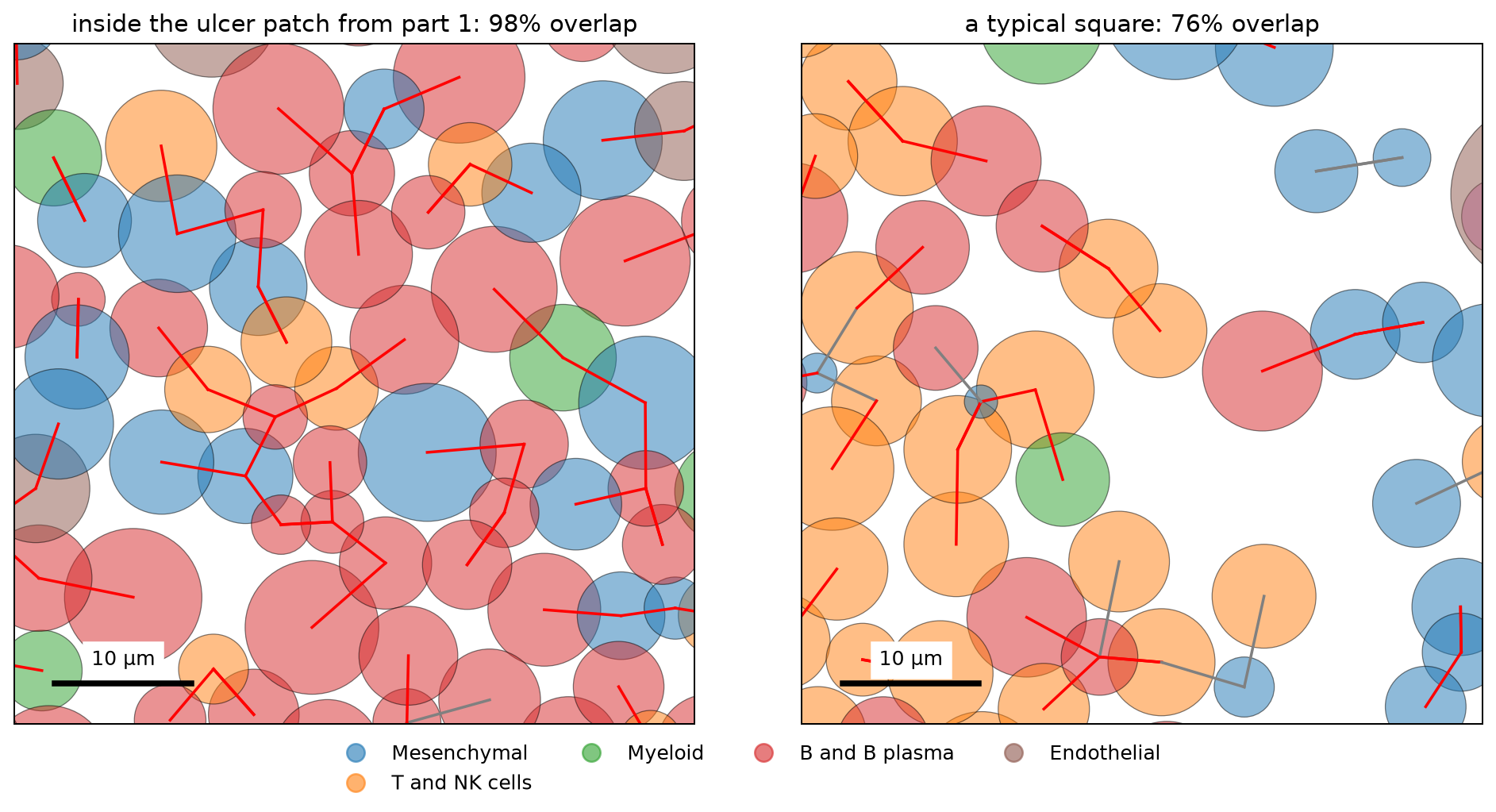
inside the ulcer patch from part 1: 58 cells, 98% overlap their nearest cell
a typical square: 38 cells, 76% overlap their nearest cellInside the ulcer, almost every cell touches its nearest cell, and many touch a cell of another type. The typical square is looser, but most lines are still red.
Checking the circles against real outlines
Figure 4 draws the cells as circles, so it can't show whether the real cells touch. For that we need a sample with its stain images and outlines. 10x Genomics shares one that was made the same way as this atlas, Xenium Prime FFPE Human Skin. It is a section of skin melanoma, run with the same Xenium Prime 5K panel (all 5,001 genes of the atlas, plus five more) and the same three-stain segmentation. It is a different tissue, but its cells are packed in a similar way. The median distance to the nearest cell is 7.1 µm, and the median cell diameter is 8.8 µm, compared with 6.1 µm and 7.4 µm in the atlas.
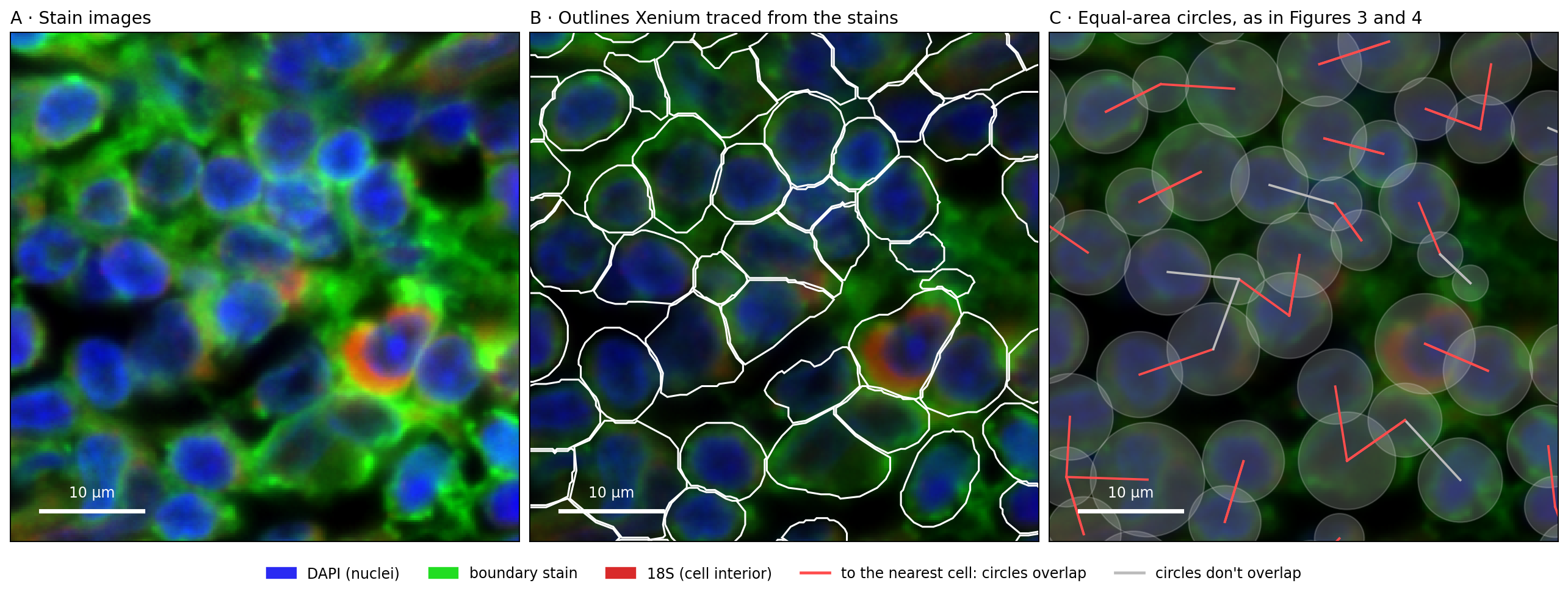
The code below runs our circle test on all 112,551 cells of the sample. Then it runs the same test with the real outlines, and calls two outlines touching when they are less than 0.25 µm apart, about one pixel of the stain images. Last, it draws one 50 µm square in Figure 5. Panel A shows the stain images, panel B adds the outlines that Xenium traced from them, and panel C draws the same cells as equal-area circles, as we did for the atlas. The sample's files are listed under Reproduce:
Show code: circles against real outlines (skin sample)
import shapely
import tifffile
import zarr
from matplotlib.patches import Polygon

# the folder with the downloaded files (see Reproduce); every file name starts with the sample name
sample = "Xenium_Prime_Human_Skin_FFPE"
skin_cells = pd.read_parquet(f"{sample}/{sample}_cells.parquet")
outlines = pd.read_parquet(f"{sample}/{sample}_cell_boundaries.parquet")

# the outlines come as one row per corner (in µm); join each cell's corners into a polygon,
# in the same order as the cell table
corners = {c: g[["vertex_x", "vertex_y"]].to_numpy() for c, g in outlines.groupby("cell_id", sort=False)}
skin_ids = skin_cells.cell_id.to_numpy()
polygon = np.array([shapely.polygons(corners[c]) for c in skin_ids], dtype=object)

# the same test as for the atlas: the nearest cell, and whether the equal-area circles overlap
# (one section, so one tree)
sxy = skin_cells[["x_centroid", "y_centroid"]].to_numpy()
sr = np.sqrt(skin_cells.cell_area.to_numpy() / np.pi)
dist, j = cKDTree(sxy).query(sxy, k=2)
snn, sd = j[:, 1], dist[:, 1]
circles = sd < sr + sr[snn]
# the test the atlas doesn't allow: are the real outlines of the two cells less than 0.25 µm apart?
touch = shapely.distance(polygon, polygon[snn]) <= 0.25

print(f"{len(skin_cells):,} cells; median distance to the nearest cell {np.median(sd):.1f} µm, "
      f"median diameter {np.median(2 * sr):.1f} µm")
print(f"circles overlap: {circles.mean():.0%}; outlines touch: {touch.mean():.0%}; "
      f"the two agree for {(circles == touch).mean():.0%} of cells")
print(f"when the circles overlap, the outlines touch {touch[circles].mean():.0%} of the time; "
      f"when they don't, {touch[~circles].mean():.0%}")

# the stain images for one 50 µm square: pixel = µm / 0.2125; channels 0-2 are DAPI (nuclei),
# the boundary stain, and 18S (the cell interior)
x0, y0, w, px = 8400, 1600, 50, 0.2125
image = zarr.open(tifffile.imread(f"{sample}/morphology_focus/morphology_focus_0000.ome.tif",
                                  aszarr=True), mode="r")["0"]
crop = np.asarray(image[:3, round(y0 / px):round((y0 + w) / px),
                        round(x0 / px):round((x0 + w) / px)]).astype(float)
# scale each stain from its 1st to its 99.7th percentile, so that faint and bright stains both show
lo, hi = np.percentile(crop, [1, 99.7], axis=(1, 2))
dapi, boundary, interior = np.clip((crop - lo[:, None, None]) / (hi - lo)[:, None, None], 0, 1)
# red: 18S, green: boundary stain, blue: DAPI
rgb = np.dstack([0.85 * interior, boundary, 0.95 * dapi])
extent = [x0, x0 + w, y0 + w, y0]

# the cells in the square, and the cells around it (so that circles at the edge are complete)
def in_box(margin):
    return np.flatnonzero((sxy[:, 0] >= x0 - margin) & (sxy[:, 0] < x0 + w + margin) &
                          (sxy[:, 1] >= y0 - margin) & (sxy[:, 1] < y0 + w + margin))
inside, around = in_box(0), in_box(12)
print(f"the square: {len(inside)} cells")

fig, axes = plt.subplots(1, 3, figsize=(15, 5.6), layout="constrained")
# A: the stain images; B: the outlines on a darker copy; C: the circles on a darker copy still
axes[0].imshow(rgb, extent=extent)
axes[1].imshow(rgb * 0.55, extent=extent)
for i in around:
    axes[1].add_patch(Polygon(corners[skin_ids[i]], fill=False, edgecolor="white", lw=1.3))
axes[2].imshow(rgb * 0.35, extent=extent)
for i in around:
    axes[2].add_patch(Circle(sxy[i], sr[i], facecolor="white", alpha=0.18, edgecolor="white", lw=1))
# a line from each cell in the square to its nearest cell: red if the circles overlap
for i in inside:
    axes[2].plot(sxy[[i, snn[i]], 0], sxy[[i, snn[i]], 1], lw=1.6,
                 color="#ff4d4d" if circles[i] else "#bbbbbb")
titles = ["A · Stain images", "B · Outlines Xenium traced from the stains",
          "C · Equal-area circles, as in Figures 3 and 4"]
for ax, title in zip(axes, titles):
    ax.set_xlim(x0, x0 + w)
    ax.set_ylim(y0 + w, y0)
    ax.set_xticks([])
    ax.set_yticks([])
    ax.set_title(title, loc="left")
    # a 10 µm scale bar
    ax.plot([x0 + 3, x0 + 13], [y0 + w - 3, y0 + w - 3], color="white", lw=3)
    ax.text(x0 + 8, y0 + w - 4, "10 µm", ha="center", va="bottom", color="white")
handles = [plt.Rectangle((0, 0), 1, 1, color=c) for c in ("#2a2af2", "#22dd22", "#d92a2a")]
handles += [plt.Line2D([0], [0], color=c, lw=2) for c in ("#ff4d4d", "#bbbbbb")]
fig.legend(handles, ["DAPI (nuclei)", "boundary stain", "18S (cell interior)",
                     "to the nearest cell: circles overlap", "circles don't overlap"],
           loc="outside lower center", ncol=5, frameon=False)
plt.show()Figure 5. Packed cells in the stain images: real outlines and equal-area circles, in a public skin melanoma sample
112,551 cells; median distance to the nearest cell 7.1 µm, median diameter 8.8 µm
circles overlap: 82%; outlines touch: 83%; the two agree for 87% of cells
when the circles overlap, the outlines touch 93% of the time; when they don't, 40%
the square: 41 cellsIn panel B, the outlines of neighboring cells run side by side, less than one pixel (0.2 µm) apart. So the real cells do touch, along an edge, and an RNA molecule detected near that edge can be counted for either cell.
Across the whole sample, 82% of cells have a circle that overlaps their nearest cell's circle, and 83% have an outline that touches their nearest cell's outline. The two tests agree for 87% of cells. When the circles overlap, the outlines touch 93% of the time. The circle test also misses some contacts: when the circles don't overlap, the outlines still touch 40% of the time. So in a sample made the same way as the atlas, the circles give about the same share of touching cells as the real outlines do.
Are neighbors the same cell type?
An RNA molecule counted for the wrong cell matters most when the two cells are different types. If an RNA molecule made by one T cell is counted for the T cell next to it, little changes, because the two cells make the same genes. If an RNA molecule made by an epithelial cell, such as EPCAM, is counted for a T cell, the T cell now holds an epithelial gene, as in Figure 1C. So for each cell that overlaps its nearest neighbor, let's check whether the neighbor is the same type. We use the 7 broad types from part 1, and the authors' 54 finer types.
To tell whether a share is high or low, we need a baseline. We shuffle the labels within each
section: every section keeps the same number of cells of each type, but the types are placed at
random. The share after shuffling is what we would see if cell types were mixed at random in the
tissue. The code below compares each cell's type with the type of its nearest neighbor, using the
row numbers in nn from step 1. It does this for the real labels and for the shuffled ones:
Show code: compare each cell's type with its nearest neighbor's
# each cell's broad and finer type, and whether it overlaps its nearest neighbor (True/False)
types = cells.cell_type.to_numpy()
fine = cells.fine_type.to_numpy()
over = cells.overlaps.to_numpy()

# baseline: shuffle the labels within each section, so the cell types keep their numbers
# but are placed at random
rng = np.random.default_rng(0)
def shuffle(labels):
    out = labels.copy()
    for section, rows in cells.groupby("section").indices.items():
        out[rows] = rng.permutation(labels[rows])
    return out

# among cells that overlap their nearest neighbor: how often is the neighbor a different type?
for name, labels in [("7 broad types", types), ("54 finer types", fine)]:
    # labels[nn] is the type of each cell's nearest neighbor; [over] keeps the overlapping cells
    differ = labels[over] != labels[nn][over]
    s = shuffle(labels)
    differ_random = s[over] != s[nn][over]
print(f"{name}: different type {differ.mean():.0%}, if placed at random {differ_random.mean():.0%}")7 broad types: different type 51%, if placed at random 77%
54 finer types: different type 67%, if placed at random 89%Half of the overlapping neighbors are a different broad type, and two thirds are a different finer type. Both shares are well below the random baseline of 77% and 89%, so cells of the same type are found together more often than chance. Even so, for one cell in two, the cell it touches is a different type. To see which types these are, the next block does two things, and Figure 6 draws both. First, for each broad type, it gives the share of its touching neighbors that are a different type, next to the same share with the types placed at random. Second, it lists the most common pairs of different types:
Show code: which cell types sit next to a different type
# for each broad type: the share of its overlapping neighbors that are a different type
differ = pd.Series(types[over] != types[nn][over], index=types[over])
by_type = differ.groupby(level=0).mean().sort_values()
print(by_type.round(2))

# the same share with the types placed at random (shuffled within each section)
s = shuffle(types)
by_type_random = pd.Series(s[over] != s[nn][over], index=s[over]).groupby(level=0).mean()

# the most common pairs of different types, as a share of all such pairs
# a: the type of each overlapping cell, b: the type of its neighbor; we keep pairs where they differ
# and sort each pair by name, so "Myeloid + T" and "T + Myeloid" count as the same pair
a, b = types[over], types[nn][over]
pairs = pd.Series([" + ".join(sorted(p)) for p in zip(a[a != b], b[a != b])])
top = pairs.value_counts(normalize=True).head(5)
print(top.round(2))

fig, (left, right) = plt.subplots(1, 2, figsize=(12, 3.6), layout="constrained")

# left: one bar per type; the black tick is the share if the types were placed at random
left.barh(by_type.index, by_type, color="C0", label="observed")
left.scatter(by_type_random[by_type.index], by_type.index, color="black", marker="|", s=300,
             label="if placed at random")
left.set_xlim(0, 1)
left.set_xlabel("share of touching neighbors that are a different type")
left.legend(frameon=False, loc="lower center", bbox_to_anchor=(0.5, 1.0), ncol=2)

# right: the five most common pairs, the most common at the top
right.barh(top.index[::-1], top[::-1], color="gray")
right.set_xlabel("share of all touching pairs of different types")
plt.show()Figure 6. Which cell types touch a different type
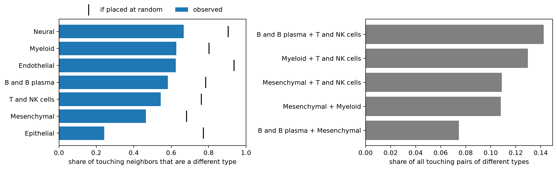
Epithelial        0.24
Mesenchymal       0.47
T and NK cells    0.54
B and B plasma    0.58
Endothelial       0.63
Myeloid           0.63
Neural            0.67
dtype: float64
B and B plasma + T and NK cells    0.14
Myeloid + T and NK cells           0.13
Mesenchymal + T and NK cells       0.11
Mesenchymal + Myeloid              0.11
B and B plasma + Mesenchymal       0.07
Name: proportion, dtype: float64In Figure 6, every bar falls short of its tick, so every type touches its own kind more often than chance. Epithelial cells touch a different type least often, 24% of the time against 77% at random, the largest gap of any type. This is probably because they form a continuous sheet, the lining of the gut. Every other type touches a different type about half the time or more. The most common mixed pairs are immune cells with each other, and immune cells with mesenchymal (stromal) cells. That is the mix we saw in the ulcer in part 1.
Do cells hold genes from the cells next to them?
So far we have measured distances. Now let's look at the counts. If RNA molecules made by an epithelial cell (its dots) are counted for the cell next to it, as in Figure 1C, then cells close to an epithelial cell will hold some EPCAM RNA, even when they are T cells or fibroblasts, which don't make EPCAM. Cells far from any epithelial cell should hold almost none.
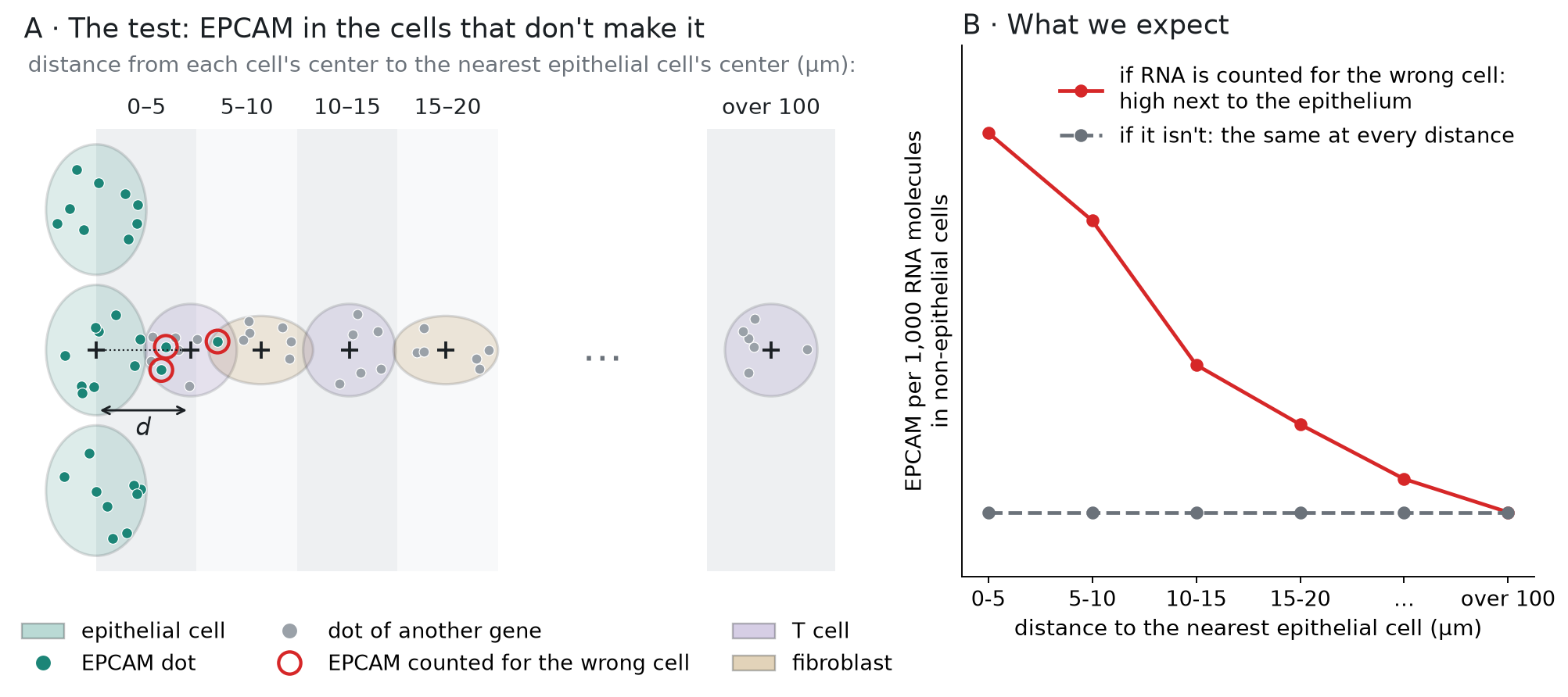
Figure 7 shows the test. For each non-epithelial cell, we measure the distance d from its center to the center of the nearest epithelial cell, and put the cell into a distance group: 0–5 µm, 5–10 µm, and so on, up to over 100 µm. In each group, we measure how much of the cells' RNA is EPCAM. If RNA is counted for the wrong cell, EPCAM will be highest in the closest group and fall with distance (panel B, red line). If it isn't, EPCAM will be about the same in every group (gray line):
Figure 7. How we test it: EPCAM in non-epithelial cells, by distance to the nearest epithelial cell
Besides EPCAM, we read one marker gene for each of the other six broad cell types, for later:
CD3E (T cells), MZB1 (plasma cells), CLDN5 (endothelial cells, which line the blood vessels), SOX10
(glial cells, in the neural type), CD163 (macrophages, in the myeloid type), and PDGFRA (fibroblasts,
in the mesenchymal type). In part 1 we read the counts of all genes for the cells in one patch. Here we need every cell but only seven genes. The matrix is stored in a compact form that
keeps only the nonzero entries, 346 million of them, since 96.8% of the entries are 0 (Figure 2).
For each nonzero entry, it stores the gene and the count, and a third array, indptr, says where
each cell's entries begin. We read the entries in chunks, keep the ones for our seven genes, and find
the cell that each one belongs to. It takes a few seconds:
Show code: read the counts of seven marker genes for every cell
markers = ["EPCAM", "CD3E", "MZB1", "CLDN5", "SOX10", "CD163", "PDGFRA"]
genes = f["var"]["_index"].asstr()[:]

# lookup[column] is 0-6 for the seven marker genes (their place in `markers`), and -1 for all others
lookup = np.full(len(genes), -1)
for k, g in enumerate(markers):
    lookup[np.flatnonzero(genes == g)[0]] = k

# the matrix is stored row by row (CSR): for each nonzero entry, its gene (indices) and its
# count (data); indptr says where each cell's entries start
X = f["layers"]["counts"]
indptr = X["indptr"][:]
# the result: one row per cell, one column per marker gene
counts = np.zeros((len(cells), len(markers)), dtype=np.int32)

# read 50 million entries at a time, so the chunk fits in memory
step = 50_000_000
for start in range(0, indptr[-1], step):
    # the gene (column number) of each entry in this chunk
    idx = X["indices"][start:start + step]
    # the entries that belong to a marker gene
    keep = np.flatnonzero(lookup[idx] >= 0)
    # the cell of each kept entry: the last cell whose entries begin at or before it
    cell = np.searchsorted(indptr, start + keep, side="right") - 1
    # copy the counts into the cell's row, in the marker gene's column
    counts[cell, lookup[idx[keep]]] = X["data"][start:start + step][keep]

# total dots of each marker gene, over all cells
print(pd.Series(counts.sum(axis=0), index=markers))EPCAM 492654
CD3E 401696
MZB1 592874
CLDN5 115718
SOX10 34845
CD163 160210
PDGFRA 246325
dtype: int64Next, for every cell, we need the distance to the nearest epithelial cell, center to center. It is
the same search as in step 1, but this time the tree holds only the epithelial cells, and we ask it
about every cell. We write it as a function, distance_to, because we reuse it for the other cell
types in Figure 9:
Show code: distance from each cell to the nearest epithelial cell
def distance_to(kind):
    # distance from each cell's center to the nearest cell of one type, in the same section
    d = np.zeros(len(cells))
    is_kind = (cells.cell_type == kind).to_numpy()
    for section, rows in cells.groupby("section").indices.items():
        # the tree holds this section's cells of that type; we ask it about all cells in the section
        source = rows[is_kind[rows]]
        dist, _ = cKDTree(xy[source]).query(xy[rows], k=2)
        # a cell of that type finds itself first, so it takes the second distance
        d[rows] = np.where(is_kind[rows], dist[:, 1], dist[:, 0])
    return d

cells["to_epithelial"] = distance_to("Epithelial")Now we put the non-epithelial cells into the distance groups of Figure 7, from 0–5 µm up to
over 100 µm. In each group we measure EPCAM in two ways. The first is EPCAM molecules per 1,000 RNA
molecules: we add up the EPCAM dots of all cells in the group, and divide by all their dots, of every
gene. Each dot is one RNA molecule, so this is the share of the group's RNA that is EPCAM. It
corrects for cell size, since a big cell holds more RNA of every gene (as in part 1). The second is
the share of cells with at least one EPCAM molecule. We also write the first measure as a function, by_distance,
because the checks below reuse it:
Show code: EPCAM in non-epithelial cells, by distance
# the distance groups, in µm
bins = [0, 5, 10, 15, 20, 30, 50, 100, np.inf]
bin_names = ["0-5", "5-10", "10-15", "15-20", "20-30", "30-50", "50-100", "over 100"]
dots = cells.dots.to_numpy()

def by_distance(values, distance, keep):
    # dots of one gene (or probe) per 1,000 dots, that is, per 1,000 RNA molecules,
    # for the cells in `keep`, by distance (µm);
    # pd.cut puts each cell into its distance group
    t = pd.DataFrame({"µm": pd.cut(distance[keep], bins, labels=bin_names),
                      "n": values[keep], "dots": dots[keep]})
    g = t.groupby("µm", observed=True)
    return 1000 * g.n.sum() / g.dots.sum()

# each cell's EPCAM dots, whether it is epithelial, and its distance to the nearest epithelial cell
epcam = counts[:, markers.index("EPCAM")]
epi = (cells.cell_type == "Epithelial").to_numpy()
near = cells.to_epithelial.to_numpy()

# the non-epithelial cells (~epi means "not epithelial"), grouped by distance
t = pd.DataFrame({"µm": pd.cut(near[~epi], bins, labels=bin_names),
                  "epcam": epcam[~epi], "dots": dots[~epi]})
g = t.groupby("µm", observed=True)
table = pd.DataFrame({"cells": g.size(),
                      "EPCAM per 1,000 molecules": 1000 * g.epcam.sum() / g.dots.sum(),
                      "share with an EPCAM dot": g.epcam.apply(lambda x: (x > 0).mean())})
print(table.round(3))
# for comparison: the epithelial cells' own EPCAM level
print(f"epithelial cells themselves: {1000 * epcam[epi].sum() / dots[epi].sum():.1f} EPCAM per 1,000 molecules") cells EPCAM per 1,000 molecules share with an EPCAM dot
µm
0-5 28389 0.799 0.062
5-10 169538 0.404 0.040
10-15 169454 0.119 0.015
15-20 159969 0.079 0.011
20-30 271761 0.059 0.009
30-50 383895 0.044 0.008
50-100 449823 0.036 0.008
over 100 252236 0.033 0.009
epithelial cells themselves: 8.1 EPCAM per 1,000 moleculesNon-epithelial cells within 5 µm of an epithelial cell hold 0.80 EPCAM molecules per 1,000 RNA molecules. Beyond 100 µm they hold 0.033, so the closest cells hold about 24 times more. The level halves from 0–5 µm to 5–10 µm, and by 10–15 µm, about two cell diameters away, it is down to 0.12. In the closest group, 6% of the cells hold at least one EPCAM molecule, compared with under 1% far away. The amount is still small. Epithelial cells themselves hold 8.1 EPCAM molecules per 1,000, so the closest non-epithelial cells hold about a tenth of that.
Three other explanations
Before we read this as RNA counted for the wrong cell, let's test three other explanations:
- Wrong labels. Some cells labeled as T cells or fibroblasts near the epithelium could really be epithelial cells, with their own EPCAM. If so, the pattern should weaken when we keep only the cells whose label the authors' classifier was sure of.
- Background. Some dots don't come from RNA molecules at all. They are background noise. If the tissue near the epithelium has more noise, the dots of every gene would rise there. Xenium's negative-control probes match no human gene, so their dots measure the noise.
- The region. Cells near the epithelium are in a different part of the gut wall. If that region raises gene counts in general, other genes would rise there too. MZB1, a plasma-cell gene, tests this in cells that are neither epithelial nor B or plasma cells.
Each check is the same measure as before, molecules per 1,000 RNA molecules by distance to the
nearest epithelial cell, with by_distance. Only the gene we count (or the control probes), or the
cells we keep, change. In the table below, each column is one check:
Show code: three checks
# MZB1 dots; cells whose label is at least 99% sure; and cells that are not B or plasma cells
mzb1 = counts[:, markers.index("MZB1")]
confident = cells.confidence.to_numpy() >= 0.99
not_b = (cells.cell_type != "B and B plasma").to_numpy()

# one column per check; & means "and", so ~epi & confident keeps confident non-epithelial cells
checks = pd.DataFrame({
    # 1. only cells whose label the classifier is at least 99% sure of
    "EPCAM, confident labels": by_distance(epcam, near, ~epi & confident),
    # 2. negative-control probes, which match no gene
    "control probes": by_distance(cells.controls.to_numpy(), near, ~epi),
    # 3. a plasma-cell gene, in cells that are neither epithelial nor B/plasma
    "MZB1": by_distance(mzb1, near, ~epi & not_b),
})
print(checks.round(3)) EPCAM, confident labels control probes MZB1
µm
0-5 0.720 0.021 0.285
5-10 0.360 0.024 0.342
10-15 0.103 0.022 0.372
15-20 0.070 0.019 0.369
20-30 0.053 0.018 0.333
30-50 0.041 0.016 0.334
50-100 0.034 0.014 0.340
over 100 0.031 0.013 0.337To compare the checks with EPCAM, Figure 8 draws them together. Each line is divided by its own level beyond 100 µm, so every line ends at 1 on the right, and a point at 20 means 20 times the far-away level. A line that stays near 1 doesn't rise near the epithelium. The y-axis is on a log scale, so that a 20-fold rise and a 2-fold rise both fit:
Show code: draw the three checks
# EPCAM in all non-epithelial cells (from the table above), next to the three checks
lines = pd.concat([table["EPCAM per 1,000 molecules"].rename("EPCAM, all labels"), checks], axis=1)

# each gene in the color of the cell type that makes it, as in Figures 4 and 9
epi_color, b_color = colors["Epithelial"], colors["B and B plasma"]
fig, ax = plt.subplots(figsize=(7, 4))
for name, color, style in [("EPCAM, all labels", epi_color, "-"), ("EPCAM, confident labels", epi_color, "--"),
                           ("control probes", "gray", "-"), ("MZB1", b_color, "-")]:
    # divide by the level far away (over 100 µm, the last group), so every line ends at 1
    level = lines[name] / lines[name].iloc[-1]
    # the legend gives each line's rise at 0-5 µm
    ax.plot(range(len(level)), level, color=color, ls=style, marker="o",
            label=f"{name}: {level.iloc[0]:.1f}× at 0-5 µm")
ax.axhline(1, color="black", lw=0.8)
ax.set_xticks(range(len(bin_names)), bin_names)
ax.set_yscale("log")
ax.set_yticks([0.5, 1, 2, 5, 10, 20], ["0.5", "1", "2", "5", "10", "20"])
ax.set_xlabel("distance to the nearest epithelial cell (µm)")
ax.set_ylabel("per 1,000 RNA molecules, relative to far away")
ax.legend(frameon=False, fontsize=9)
plt.show()Figure 8. Only EPCAM rises next to epithelial cells: EPCAM against three checks, by distance
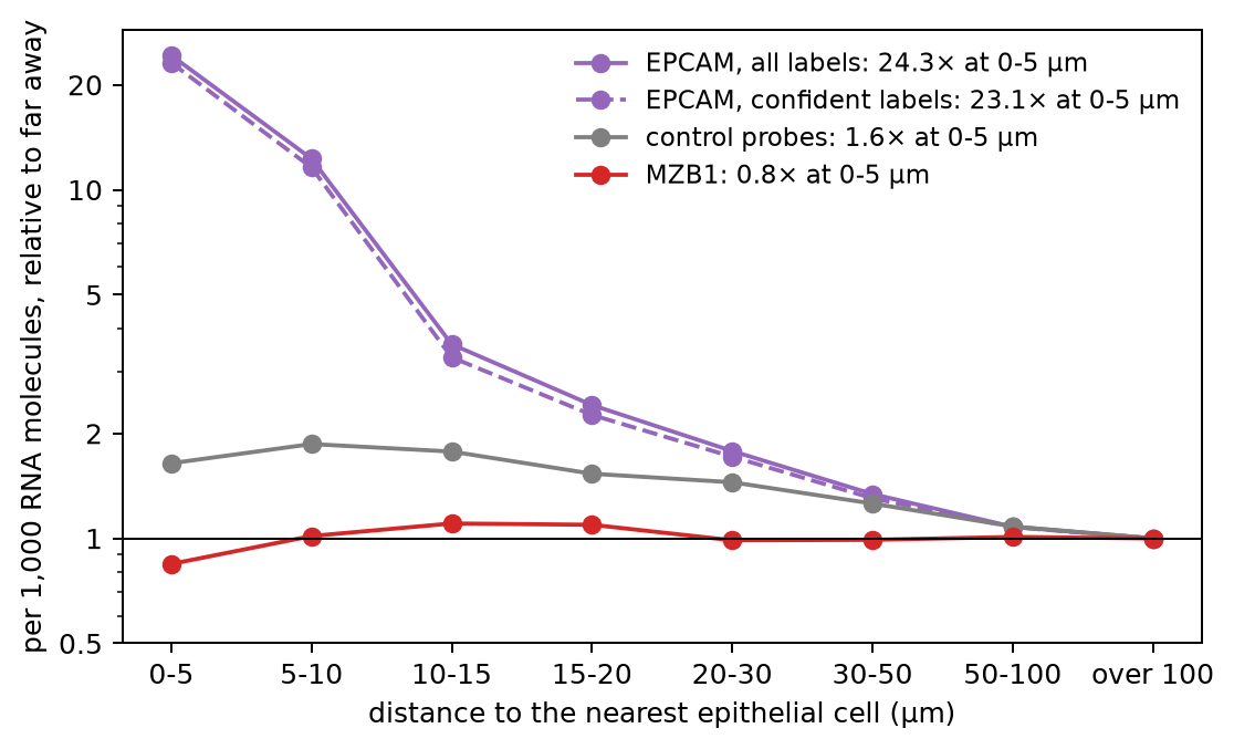
The checks rule out all three:
- With confident labels only (99% or more), EPCAM is still 0.72 per 1,000 within 5 µm and 0.031 beyond 100 µm, about 23 times more.
- The control probes rise from 0.013 to 0.021 per 1,000 near the epithelium, less than 2-fold, compared with about 24-fold for EPCAM.
- MZB1 stays between 0.28 and 0.37 per 1,000 at every distance from the epithelium, and it is lowest right next to it.
So EPCAM rises in the cells next to epithelial cells because of the epithelial cells, and most of the rise is within one or two cell diameters.
One marker gene for each cell type
Figure 9 repeats the measure for all seven marker genes. Marker genes are rarely made by one cell type alone, so first we check how specific each one is. For each broad type, we tried a few well-known marker genes from the panel and kept the one with the largest share of its RNA in that type. Panel A shows these shares. Each row is one gene, each column is one cell type, and each number is the share of the gene's RNA molecules counted for cells of that type. Panel B is drawn the same way as Figure 8. For each gene, we keep the cells of all other types, measure the distance to the nearest cell of the type that makes it, and divide the level by the level beyond 100 µm:
Show code: draw the seven genes
# each marker gene, with the cell type that makes it (in the order of `markers`)
sources = {"EPCAM": "Epithelial", "CD3E": "T and NK cells", "MZB1": "B and B plasma",
           "CLDN5": "Endothelial", "SOX10": "Neural", "CD163": "Myeloid", "PDGFRA": "Mesenchymal"}
source_types = list(sources.values())

# A: the share of each gene's RNA molecules in each cell type, in %
# (sum each gene's dots over the cells of each type, then divide by the gene's total)
per_type = pd.DataFrame(counts, columns=markers).groupby(cells.cell_type.to_numpy()).sum()
share = (100 * per_type / per_type.sum()).T.loc[markers, source_types]

# B: each gene in the cells of all other types, by distance to the nearest cell of its own type
rise = {}
fig, (left, right) = plt.subplots(1, 2, figsize=(13, 4.6), layout="constrained",
                                  gridspec_kw=dict(width_ratios=[1, 1.35]))
for gene, kind in sources.items():
    other = (cells.cell_type != kind).to_numpy()
    level = by_distance(counts[:, markers.index(gene)], distance_to(kind), other)
    # divide by the level far away (over 100 µm, the last group), so every line ends at 1
    level = level / level.iloc[-1]
    rise[gene] = level.iloc[0]
    # the same color for each type as in Figure 4
    right.plot(range(len(level)), level, marker="o", color=colors[kind],
               label=f"{gene}, from {kind}: {level.iloc[0]:.0f}× at 0-5 µm")
print(pd.DataFrame({"made by": source_types, "% of its RNA in that type": np.diag(share),
                    "rise at 0-5 µm": list(rise.values())}, index=markers).round(1))

# A: the shares as a grid; the diagonal is each gene in its own type
left.imshow(share, cmap="Blues", vmin=0, vmax=100)
for i in range(len(markers)):
    for j in range(len(source_types)):
        left.text(j, i, f"{share.iloc[i, j]:.0f}", ha="center", va="center", fontsize=9,
                  color="white" if share.iloc[i, j] > 50 else "black")
left.set_xticks(range(len(source_types)), source_types, rotation=40, ha="right")
left.set_yticks(range(len(markers)), markers)
left.set_title("A · share of each gene's RNA, by cell type (%)", loc="left")

right.axhline(1, color="black", lw=0.8)
right.set_xticks(range(len(bin_names)), bin_names)
right.set_yscale("log")
right.set_yticks([1, 2, 5, 10, 20, 40], ["1", "2", "5", "10", "20", "40"])
right.set_xlabel("distance to the nearest cell that makes the gene (µm)")
right.set_ylabel("per 1,000 RNA molecules, relative to far away")
right.set_title("B · in the cells of other types, by distance", loc="left")
right.legend(frameon=False, fontsize=9)
plt.show()Figure 9. One marker gene per cell type: how specific each one is, and its RNA in other cell types by distance
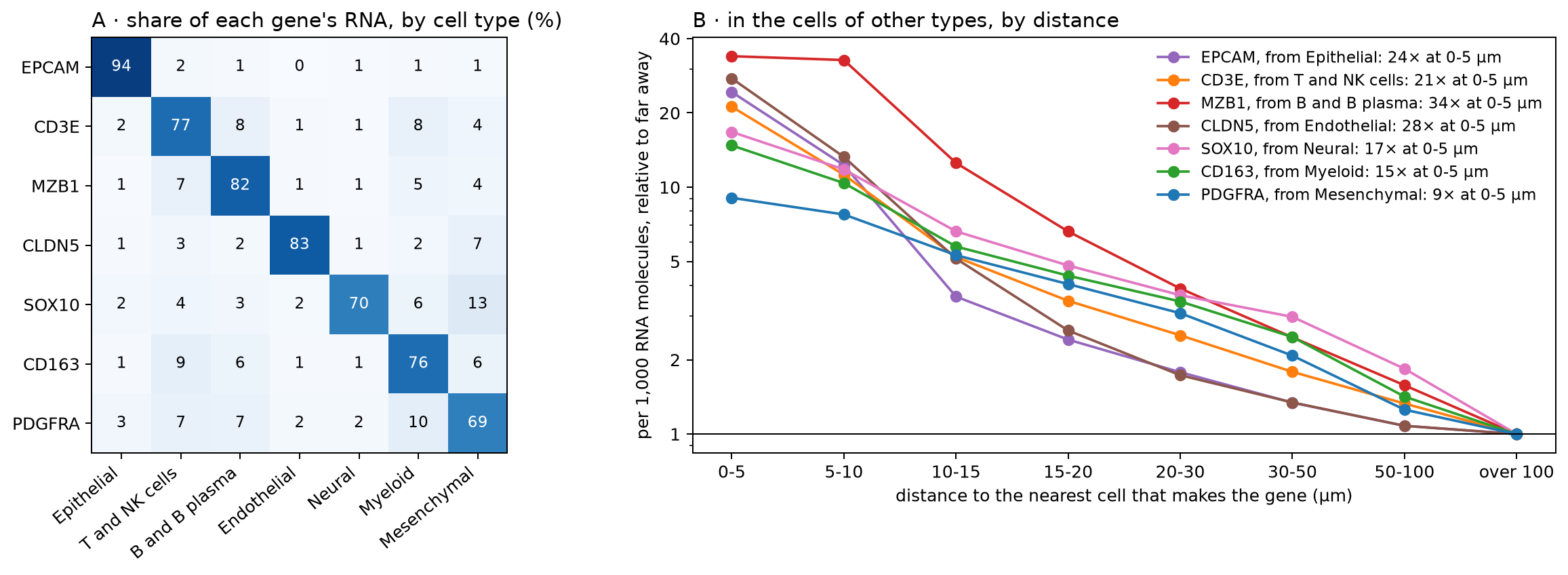
               made by  % of its RNA in that type  rise at 0-5 µm
EPCAM       Epithelial                       94.2            24.3
CD3E    T and NK cells                       76.8            21.2
MZB1    B and B plasma                       81.9            33.9
CLDN5      Endothelial                       83.3            27.6
SOX10           Neural                       69.6            16.7
CD163          Myeloid                       76.2            14.8
PDGFRA Mesenchymal 69.4 9.1In panel A, the diagonal runs from 69% (PDGFRA in mesenchymal cells) to 94% (EPCAM in epithelial cells). The other 6% to 31% of each gene's RNA is spread over the other types, at most 13% in any one. Some of it is real, since a few cells of other types make the gene too. Some of it is RNA counted for the wrong cell, which panel B measures. Panel A can't tell the two apart.
In panel B, all seven genes show the same pattern as EPCAM. Within 5 µm of the cells that make them, cells of other types hold 9 to 34 times the level found far away, and most of that falls off within 10–15 µm. MZB1 stays high out to 10 µm. Plasma cells are often found in dense groups, so a cell 5–10 µm from one plasma cell is probably close to others too. PDGFRA rises least, 9-fold. Mesenchymal cells are the most common type, so only 15,350 cells of other types are more than 100 µm from one, and they may not be typical. Beyond 20 µm, all lines decline slowly. Part of that slow decline may come from differences between regions of the tissue, since the control probes also drift with distance, by less than 2-fold.
These numbers can't tell us how an RNA molecule ended up in the wrong cell. A misplaced edge between two outlines (Figure 1C), two cells stacked in the depth of the 5 µm section (part 1), and RNA molecules that moved a few µm during processing all have the same result. The molecule lies inside the outline of the cell next to the one that made it, so it is counted for that cell. To tell these apart, we would need the dots (where each RNA molecule was detected) and the outlines.
Does it change what we learn about T cells?
Spatial atlases are often used to ask how a cell type changes with its surroundings. For example, do T cells next to the epithelium differ from T cells deeper in the tissue? Let's ask it the simple way, and look at which genes come out on top. We take the T cells within 10 µm of an epithelial cell (near) and the T cells more than 50 µm away (far). For every gene, we add up its RNA molecules in each group and compare the two levels, per 1,000 RNA molecules as before.
We make this comparison inside each tissue section, and then take the median over the sections. The sections come from different patients, and some are inflamed and some are not. If we put the T cells of all sections into two groups, these differences mix into the comparison. For example, 38% of all far T cells come from one inflamed section, but only 2% of the near T cells do. Inside one section, near and far T cells share the patient and the tissue, so the main difference left is their distance to the epithelium. We keep the sections with at least 300 T cells in each group. Figure 10 shows the whole comparison, with made-up cells and numbers:
Figure 10. How we compare T cells near the epithelium with T cells far from it
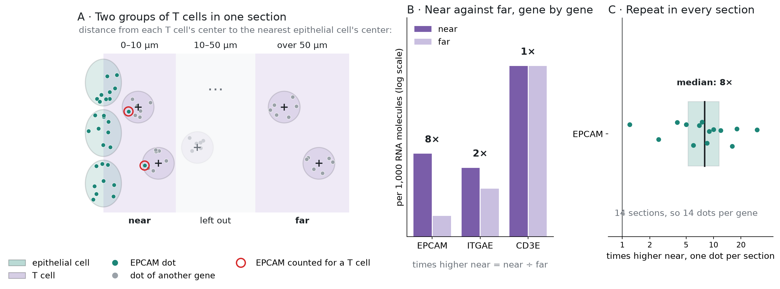
In panel B, a gene that the T cells make the same way everywhere, such as CD3E, is at the same level in both groups (1 times). A gene from the epithelial cells next door, such as EPCAM, is higher in the near group. Panel C repeats this in every section, so each gene gets one fold change per section.
For each gene, we also note how much of its RNA in the whole atlas is counted for epithelial cells. All of this takes one more pass over the count matrix, this time keeping all 5,001 genes:
Show code: compare T cells near the epithelium with T cells far from it
# the two groups: T cells within 10 µm of an epithelial cell (0), and more than 50 µm away (1)
is_t = (cells.cell_type == "T and NK cells").to_numpy()
group = np.full(len(cells), -1)
group[is_t & (near < 10)] = 0
group[is_t & (near > 50)] = 1

# T cells in each group, section by section; keep sections with at least 300 in each group
n = pd.crosstab(cells.section[group >= 0], group[group >= 0])
use = n[(n[0] >= 300) & (n[1] >= 300)].index
print(f"{len(use)} of {len(n)} sections: {n.loc[use, 0].sum():,} near and {n.loc[use, 1].sum():,} far T cells")

# a slot for each section and group: the near T cells of section k go to slot 2k, the far ones
# to slot 2k + 1; all other cells get -1
position = pd.Series(np.arange(len(use)), index=use)
slot = np.full(len(cells), -1)
kept = (group >= 0) & cells.section.isin(use).to_numpy()
slot[kept] = 2 * position[cells.section[kept]].to_numpy() + group[kept]

# the dots of every gene, added up in each slot, in the epithelial cells, and in all cells;
# we read the matrix in chunks, as before
by_slot = np.zeros((2 * len(use), len(genes)))
epi_total = np.zeros(len(genes))
all_total = np.zeros(len(genes))
for start in range(0, indptr[-1], step):
    idx = X["indices"][start:start + step]
    data = X["data"][start:start + step]
    # the cell, and the slot, of every entry in this chunk
    cell = np.searchsorted(indptr, start + np.arange(len(idx)), side="right") - 1
    sl = slot[cell]
    ok = sl >= 0
    # bincount adds up the counts for each (slot, gene) pair
    by_slot += np.bincount(sl[ok] * len(genes) + idx[ok], weights=data[ok],
                           minlength=by_slot.size).reshape(by_slot.shape)
    is_epi = epi[cell]
    epi_total += np.bincount(idx[is_epi], weights=data[is_epi], minlength=len(genes))
    all_total += np.bincount(idx, weights=data, minlength=len(genes))

# each gene per 1,000 RNA molecules in each slot; then, section by section, near over far
# (0.01 is added to both, so that a gene absent far away doesn't divide by zero)
level = 1000 * by_slot / by_slot.sum(axis=1, keepdims=True)
fold = (level[0::2] + 0.01) / (level[1::2] + 0.01)

# the median over the sections: half of the sections are above it, half below
de = pd.DataFrame({"times higher": np.median(fold, axis=0),
                   "sections higher": (fold > 1).sum(axis=0),
                   "% in epithelial cells": 100 * epi_total / all_total,
                   "dots near": by_slot[0::2].sum(axis=0).astype(int)}, index=genes)
# keep genes with at least 100 dots in the near T cells, and rank them, the highest first
de = de[de["dots near"] >= 100].sort_values("times higher", ascending=False)
de["rank"] = np.arange(1, len(de) + 1)
print(de.head(10).round(1))

# how many of the top genes are epithelial genes (most of their RNA in epithelial cells)
for n_top in [20, 50]:
    print(f"top {n_top}: {(de.head(n_top)['% in epithelial cells'] > 50).sum()} epithelial genes")
# a gene that T cells in the epithelium are known to make
print(de.loc[["ITGAE"]].round(1))14 of 16 sections: 50,587 near and 105,075 far T cells
times higher sections higher % in epithelial cells dots near rank
DEFA6 17.0 13 88.3 4866 1
EPCAM 7.6 14 94.2 4272 2
EPS8L3 5.4 14 90.0 1550 3
FCGBP 4.8 14 94.8 4518 4
CDH1 4.2 14 88.5 937 5
CDX2 4.0 13 85.6 885 6
CLDN7 4.0 14 88.6 699 7
CDX1 3.6 13 84.7 1266 8
TSPAN8 3.6 14 89.1 1133 9
KLF5 3.4 14 82.7 593 10
top 20: 20 epithelial genes
top 50: 42 epithelial genes
times higher sections higher % in epithelial cells dots near rank
ITGAE 1.9 13 11.9 2010 149Figure 11 draws the top 20 genes, and ITGAE below them, with all 14 sections of each gene. Each dot is one section. The line inside each box is the median, and the box holds the middle half of the sections. The x-axis is on a log scale, and the black line at 1 means no difference between near and far:
Show code: draw the top genes
# the top 20 genes, then ITGAE; for each, its fold change in every section (a column of `fold`)
show = pd.concat([de.head(20), de.loc[["ITGAE"]]])
column = pd.Series(np.arange(len(genes)), index=genes)
per_section = [fold[:, column[g]] for g in show.index]
# epithelial genes in the epithelial color, the T-cell gene in the T-cell color
color = [colors["Epithelial"] if share > 50 else colors["T and NK cells"]
         for share in show["% in epithelial cells"]]
# the rows from the top down, with a gap before ITGAE
y = np.r_[np.arange(20), 21.2]

fig, ax = plt.subplots(figsize=(7, 6.5))
boxes = ax.boxplot(per_section, positions=y, orientation="horizontal", widths=0.6, showfliers=False,
                   patch_artist=True)
for box, c in zip(boxes["boxes"], color):
    box.set(facecolor=c, alpha=0.35)
for median in boxes["medians"]:
    median.set(color="black")
# one dot per section, moved up or down a little at random so that the dots don't hide each other
jitter = np.random.default_rng(1)
for yi, values, c in zip(y, per_section, color):
    ax.scatter(values, yi + jitter.uniform(-0.2, 0.2, len(values)), s=10, color=c, zorder=3)
ax.axvline(1, color="black", lw=0.8)
ax.set_xscale("log")
ax.set_xticks([0.5, 1, 2, 5, 10, 20, 50, 100], ["0.5", "1", "2", "5", "10", "20", "50", "100"])
ax.set_yticks(y, [f"{g} ({r})" for g, r in zip(show.index, show["rank"])])
ax.invert_yaxis()
ax.set_xlabel("times higher in T cells near the epithelium (one dot per section)")
handles = [plt.Rectangle((0, 0), 1, 1, color=colors[t], alpha=0.6) for t in ["Epithelial", "T and NK cells"]]
ax.legend(handles, ["epithelial gene (most of its RNA in epithelial cells)", "T-cell gene"],
          frameon=False, loc="upper center", bbox_to_anchor=(0.5, -0.1), ncol=2)
plt.show()Figure 11. T cells near the epithelium, compared with T cells far from it in the same section: the top 20 genes are all epithelial genes
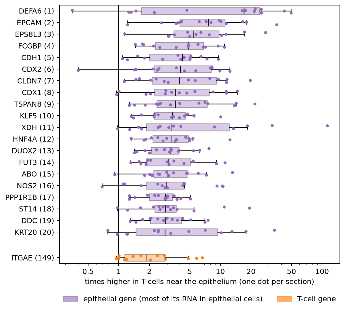
All 20 are epithelial genes. For each of them, 64% to 95% of its RNA in the atlas is counted for epithelial cells. They include EPCAM, KRT20, and E-cadherin (CDH1), DEFA6 from Paneth cells, and CDX1, CDX2, and HNF4A, which set the identity of gut epithelial cells. The medians run from 2.8 to 17 times higher near the epithelium, and each gene is higher there in 12 to 14 of the 14 sections. Of the top 50, 42 are epithelial genes. In the previous sections, we saw how such genes end up in the cells next to epithelial cells. Had we pooled all sections into two groups, the same kind of genes would come out on top, but the rises would look larger. EPCAM, for example, would look 17 times higher instead of about 8.
The boxes also show how much the sections differ. DEFA6 is 16 to 50 times higher near the epithelium in 8 sections. In the 4 sections from two of the patients, it is 0.3 to 1.5 times, so it doesn't rise there. A single number for each gene would hide this.
T cells that live in the gut lining do differ from T cells deeper in the tissue. For example, they make more ITGAE (CD103), a protein that holds them to the epithelial cells. Here ITGAE is about 2 times higher near the epithelium, in 13 of the 14 sections. It is a real difference, but it ranks 149th, below the epithelial genes. In a plain analysis, the RNA counted for the wrong cell fills the top of the list and pushes the real biology down.
We rank the genes by how many times higher they are, without a statistical test. A test would not fix this. It compares the counts, and the counts already hold the RNA from the neighboring cells.
What others have measured
Several recent studies have measured this problem in other ways:
- Spurious co-expression. Yamasaki (2026) studied the public 10x Xenium breast cancer section. In one dense region, 24.2% of the cells next to hormone-receptor-positive cells showed spurious co-expression of their genes. The study also argues that no assignment method can be fully accurate there. The best possible accuracy is about 0.66 to 0.81. It is a single-author preprint.
- Cells stacked in depth. ovrlpy (Tiesmeyer et al., Nature Biotechnology, 2026) uses the dots' depth (z) to find places where two cells lie on top of each other in the section. In a mouse brain section, it found these in about 20% of the tissue, and in more than 75% of the densest regions.
- Mixed cells. SPLIT (Bilous et al., Nature Methods, 2026) flags cells whose counts look like a mix of two cell types, and corrects their counts with a single-cell RNA reference. Across breast cancer samples, 1.6% to 54% of the cells were flagged.
- The cost downstream. cellAdmix (Mitchel et al., Nature Genetics, 2026) measured what mixed counts do to analyses of how cell types change together. In its test tissues, 25% to 30% of the top hits were false positives caused by the mixing.
Our check is simpler. It needs only the cell table and the gene counts, which most shared atlases include.
Summary and what comes next
In this atlas, cells are packed close together, and RNA made by one cell type is counted, in small amounts, for the cells that touch it. In a single cell it is little. Next to an epithelial cell, other cells hold about a tenth of the epithelial cell's own EPCAM level. But a comparison of two groups adds up thousands of cells, and then it shows. T cells next to the epithelium seem to make 20 epithelial genes, and these fill the top of the gene list, above the real changes in those T cells. We haven't tested whether this changes any of the paper's results.
- Packing. As circles of the same area, 76% of cells overlap their nearest cell (52% to 90% by section, 98% inside the ulcer). In a public sample made the same way, the real outlines give 83%.
- Cell types. Half of the touching neighbors are a different broad type.
- Counts. Next to the cells that make them, marker genes are 9 to 34 times higher in other cell types than far away. The control probes and an unrelated gene don't rise.
- Comparisons. Between T cells near the epithelium and T cells far from it, the top 20 genes are all epithelial genes. ITGAE, which T cells in the epithelium do make, ranks 149th.
To check another atlas, plot a marker gene in the other cell types against the distance to the cells that make it, next to the control probes. And before you trust the top genes of a spatial comparison, check how much of their RNA belongs to the cell types around the cells.
Baysor and cellAdmix fix the counts with the dots, which this atlas doesn't share. SPLIT works from the counts and a single-cell reference, so it could be run here. Most fixes still give each dot to one cell. Another way is to keep the uncertainty. For each dot, we would estimate the chance that it came from each nearby cell or from background noise, and carry those chances into the counts and the tests. We will try that later on a public 10x sample that includes the dots. The next note in this series goes back to the biology. It asks which cell types change in inflammation, and what the changed neighbors do to a comparison of inflamed and adjacent tissue.
Reproduce
Data. The same file as in part 1, xenium5k_scVI_CellCharter_batch2_reannot_SCP.h5ad (about
9 GB), from the study's page on the
Broad Single Cell Portal. The
download is free but needs a Google sign-in. For Figure 5, the public
Xenium Prime FFPE Human Skin sample from 10x Genomics: the files
Xenium_Prime_Human_Skin_FFPE_cells.parquet and Xenium_Prime_Human_Skin_FFPE_cell_boundaries.parquet,
and the morphology_focus/ folder from the Xenium output bundle (Xenium_Prime_Human_Skin_FFPE_xe_outs.zip,
3.1 GB). Put them in a folder named Xenium_Prime_Human_Skin_FFPE, next to the atlas file.
Environment. Python 3.9 or later, with h5py, pandas, numpy, scipy, and matplotlib (3.10 or later). For Figure 5, also pyarrow, shapely, tifffile, and zarr.
Code. Start Python in the folder that holds the file, and run the code blocks above in order, in
one session. Each block uses names defined by the blocks before it. All of them run in under a
minute. The code is in
tensoromics/notes/spatial-xenium-crohns:
| Figures | Where |
|---|---|
| 1, 3, 7, 10 | scripts/p2_schematic.py, scripts/p2_method_schematic.py, scripts/p2_test_schematic.py, and scripts/p2_de_schematic.py (drawn from made-up cells, no data needed) |
| 2 | scripts/p2_matrix_fig.py (reads the data file) |
| 4, 6, 8, 9, 11 | the code blocks above, also in spatial-transcriptomics-crohns-cell-overlap.ipynb |
| 5 | the code block above (it reads the skin sample, so the notebook leaves it out), also scripts/p2_stain_fig.py |
Working on something like this?
I take on consulting work in computational biology and AI for drug discovery. See the services or get in touch.