Single-molecule affinity proteomics has the same counting problem as RNA-seq

Why reading one protein molecule at a time lands you in a problem RNA-seq solved years ago.

Why proteins are harder to measure than RNA

RNA-seq is cheap, scalable and reliable. I think that is a big part of why we lean on it so hard. Proteins are closer to what we actually want to know, and the data on them is much thinner.

One reason is that there's no protein PCR, so you can't make more of the thing you're trying to measure. Another is that protein abundances in plasma run over something like ten orders of magnitude, and no single instrument covers that.

A third is that each RNA transcript can become many proteoforms once cleavage, truncation and post-translational modifications come in, and those combine multiplicatively. Tau, for example, has six well-established isoforms in the adult human brain. Track just seven modification sites on top of those and you already have 768 possible states, and real tau carries far more sites than seven. A single number for the gene averages over forms that do different things.

How people measure proteins today

Given all those constraints, it's really interesting to see how much ingenuity has gone into the available technologies that measure proteins.

For anything untargeted, mass spectrometry cuts proteins into peptides and measures the peptides, which loses the linkage between pieces of the same molecule along the way. It also creates an ambiguity of its own, because a peptide can belong to several proteins. SomaScan captures proteins with modified DNA aptamers and reads thousands of them by hybridisation. Olink tags pairs of antibodies with DNA oligos that join into a barcode when both bind the same protein, then amplifies and sequences it. Alamar's NULISA is also antibody-based with a nucleic-acid readout, offered with sequencing or qPCR. Seer sits in front of the instrument, using engineered nanoparticles that form a protein corona to compress the dynamic range before anything is measured, an approach now run at population scale.

Having analysed datasets from most of these, it's clear they're all strong tools aimed at specific problems, each with its own strengths and weaknesses (UK Biobank, Chinese cohort).

A different approach: single-molecule affinity mapping

I recently came across another technology, from Nautilus Biotechnology, that goes at it from a different angle: counting the different proteoforms that might be present, one molecule at a time. Nautilus calls it iterative affinity mapping and has published two versions: PrISM, for untargeted proteome-wide identification, and a targeted assay for tau.

The idea is to keep each protein whole instead of cutting it into peptides, denature it so its features are accessible, and attach it to a fixed location on a dense array, at most one molecule per location, where it stays for the whole run. Affinity probes, usually antibodies or other binding reagents that recognise a short peptide motif or a modification, are then applied one at a time. Each one flows over the array, gets time to bind, and is then washed off. After every probe the instrument records, for each molecule, whether that probe bound or not.

Because the molecule stays whole and never moves, every result in its record came from that one molecule. Features that show up together really were together on the same protein. Cutting proteins into peptides loses exactly that linkage, which is why proteoform-level questions are reachable here.

Each probe is aimed at one small feature, often a short peptide motif only a few amino acids long. Motifs like that recur across many proteins, so a probe can be perfectly specific for its motif and still not tell you which protein it just bound. We have to rely on the pattern across cycles rather than on any single binding event. That ordered list of yes/no answers for one molecule is its affinity trace. For a six-cycle run applying three probes twice each, one molecule's trace looks like this:

cycle     1   2   3   4   5   6
probe    P0  P1  P2  P0  P1  P2
call      1   0   1   1   0   0

Stack up a few of those, add a table of how each probe behaves against each candidate, and you have everything the model gets to work with:

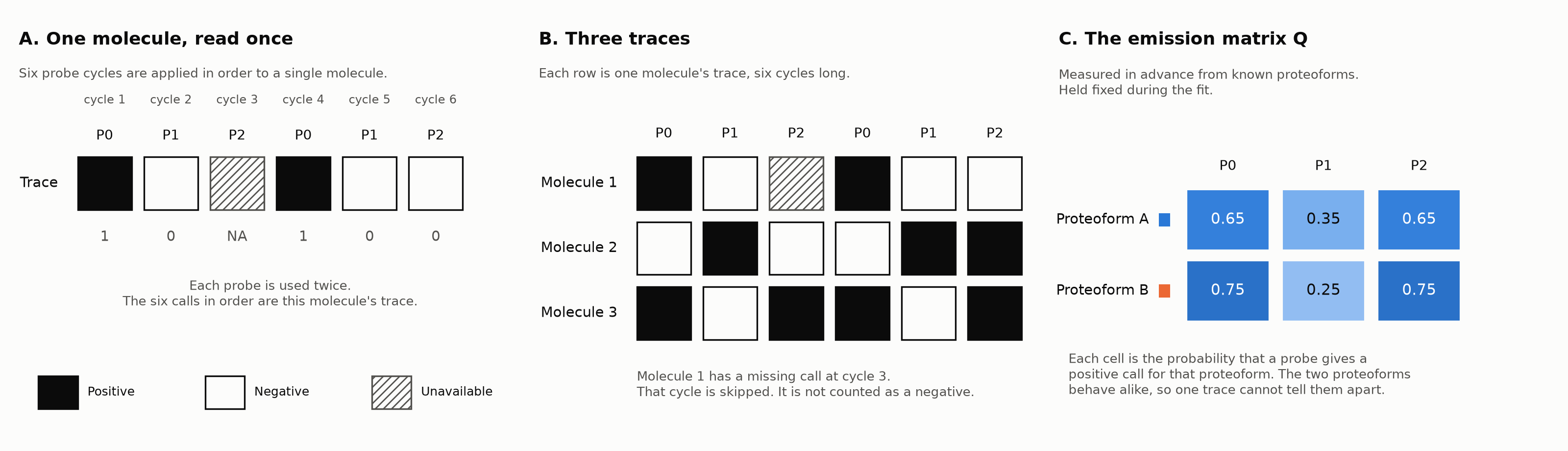
Everything the model gets is in those three panels. Nothing else about the molecule is recorded.

One yes/no answer carries very little information next to a mass spectrum, so you're leaning on many weak measurements rather than a few strong ones. Probes also bind imperfectly, missing features they should have caught and occasionally catching ones they shouldn't. So a single trace is usually consistent with several candidates and you can't tell which one produced it. Better probes won't fix that either, because the ambiguity is in the biology rather than the reagents. The approach is also much newer than the others, with far less of a track record behind it.

The technology gives you affinity traces as evidence, and turning that noisy evidence into abundances is a statistics problem. One I had seen before.

The same ambiguity in RNA-seq and mass spectrometry

If you want to know how much of each proteoform is in the sample, you have to take a pile of traces that are each consistent with several candidates, work out how to distribute them, and count.

Proteomics already has a version of this problem. When a peptide belongs to several proteins, the common shortcut is the razor-peptide rule: give it to whichever protein group already has the most evidence, and count it there. That's a hard assignment, and it throws away the same information as picking the best-matching transcript for a read.

RNA-seq stopped doing that years ago. RSEM, Salmon and kallisto share each read across the transcripts it could have come from, then iterate until the abundances settle. EMASE, which I worked on for allele-specific expression, does the same over a read-to-gene-to-isoform-to-allele tensor, so reads get split across nested levels at once rather than across a flat list. The same EM applies to shared peptides, and it applies to affinity traces.

EM is one of my favourite old-school tools in applied statistics. The paper is from 1977, and once you understand the basic idea you can't unsee where EM can solve a problem.

Here are the parallels between the two, and they're close enough that I wrote ProteoEM, an open-source implementation, to see how far they go.

RNA-seq and affinity proteomics, stage by stage

Stage by stage, the two problems line up like this:

Stage	RNA-seq	Affinity proteomics
Raw observation	Read sequence $S_i$	Probe-binding trace $Y_{i\cdot}$
Candidate reference	Transcript sequences	The candidate set: proteoforms for a targeted panel, proteins for a broadside one
Observation model	Alignment, sequencing-error and fragment-generation model	Probe sensitivity, cross-reactivity and false-negative model $Q$
Candidate likelihood	$L_{ik}=P(S_i\mid T_k)$ , the chance of seeing read $i$ if transcript $k$ produced it	$L_{ik}=P(Y_{i\cdot}\mid Z_i=k,Q)$ , the chance of seeing trace $i$ if proteoform $k$ produced it
Evidence matrix	Sparse: a read scores against a handful of transcripts, the rest are structural zeros	Dense: every candidate has a non-zero likelihood for every trace
Grouping for speed	Equivalence classes: reads that align to the same transcripts	Trace-likelihood classes: traces that score the same against every candidate
Assignment probability	$r_{ik}\propto\pi_k L_{ik}$ , the chance read $i$ came from transcript $k$	$r_{ik}\propto\pi_k L_{ik}$ , the chance trace $i$ came from proteoform $k$
Abundance inference	EM estimates transcript proportions	EM estimates proteoform proportions
Correcting the counts	Effective length, inside the M step: a longer transcript produces more reads	Observation yield, applied after the fit: the chance a molecule gives a trace you keep

The bottom rows of the table are the same for RNA-seq and for affinity proteomics. EM estimates the proportions. The assignment probability uses the same formula. Both fields can group observations that carry the same evidence, so the fit runs on fewer rows than there are observations. The likelihood has the same form as well, the probability of the observation given the candidate.

The differences are all in the top half. An aligner compares a read's sequence to a reference and decides which transcripts it matches, so the evidence arrives with the read. A trace is only a list of yes/no answers, and those mean nothing until you know how the probes behave. That knowledge comes from a separate calibration experiment, the $Q$ in the table. RNA-seq needs nothing of the kind, and affinity proteomics cannot skip it.

The shared part, then, is the estimator itself. What differs is where the likelihood comes from, what it costs to get, and how dense the resulting table is. RNA-seq gets them all easily from alignment. In affinity proteomics you have to build them.

What carries over from RNA-seq quantification

The mapping is close enough that the same estimator works on both problems. If you have ever quantified transcripts, you already understand how proteoform abundances come out of ambiguous traces: score each observation against every candidate, share it out in proportion to how well each explains it, add up the shares, and repeat.

The table hides what that upper half costs, and where borrowing the RNA-seq intuition starts to mislead rather than help. That is a longer story, and I will write it up separately.

ProteoEM is open source under an MIT licence, and the code and a synthetic benchmark are in the repo. The manuscript, which covers the model and its limits properly, should be on bioRxiv shortly.